Understanding FAISS Indexing
Understanding FAISS Indexing
https://arithmancylabs.medium.com/understanding-faiss-indexing-86ec98048bd9
In this article we will dive deep into the Facebook AI Similarity Search library, explaining how it can be used for efficient nearest neighbor search in high-dimensional spaces. We’ll cover the algorithms behind index creation and retrieval.
Introduction to FAISS
FAISS is a library developed by Meta AI Research to efficiently perform similarity search and clustering of dense vectors. It is written in C++ and is optimized for large-scale data and high-dimensional vectors with support for both CPU and GPU implementations. The central concept of FAISS is the index, a data structure used to store and search through vectors. FAISS supports several types of indexes, each designed for different trade-offs in terms of memory usage, speed and accuracy. Below we will explore the different indexing techniques- the Flat Index, Inverted File Index, HNSW Index, Product Quantization and IVFPQ.
Flat Index
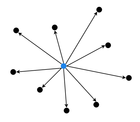
Flat Index is a simple brute-force approach where all vectors are stored and compared directly.
Algorithm
- Linear Search: Computes the distance from a query vector to every vector in the dataset and returns the nearest ones using exact distance metrics. IndexFlatL2 uses Euclidean distance, while IndexFlatIP uses the inner product (or dot product) as the distance metric.
Accuracy: 100% accurate as it exhaustively checks all vectors.
Use case: Small datasets with ≤≤ 100,000 vectors.
import faiss
import numpy as np

# Example: Creating a flat index
dimension = 128  # Dimensionality of vectors
n = 10000  # Number of vectors
vectors = np.random.rand(n, dimension).astype('float32')  # Database of vectors
query = np.random.rand(1, dimension).astype('float32')  # Query vector

index = faiss.IndexFlatL2(dimension)  # L2 distance index
index.add(vectors)  # Add vectors to index

# Searching the nearest neighbors
k = 5  # Number of neighbors to return
distances, indices = index.search(query, k)
Inverted File Index
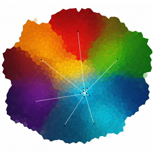
IVF divides the vector space into smaller regions (clusters). It first assigns vectors to clusters using a coarse quantizer and then performs searches within the most relevant clusters for faster retrieval.
Algorithm
- Quantization: K-means clustering to partition the data into Voronoi cells and each vector is assigned to its nearest cluster.
- Inverted File Structure: Maintains a record of the vectors and the cells to which they are assigned.
- Search Process: The distance between the query and the centroids is calculated followed by a search within the closest clusters. The distance metric could be L2 distance, dot product or cosine similarity.
Accuracy: Can be tuned by adjusting the number of clusters as a trade-off between speed and accuracy.
Use case: Suitable for large-scale datasets, balancing speed and memory usage.
quantizer = faiss.IndexFlatL2(dimension)  # Quantizer for IVF
nlist = 100  # Number of clusters
index_ivf = faiss.IndexIVFFlat(quantizer, dimension, nlist, faiss.METRIC_L2)
index_ivf.train(vectors)  # Training on the dataset
index_ivf.add(vectors)  # Add vectors after training

# Searching the nearest neighbors
k = 5
distances, indices = index_ivf.search(query, k)
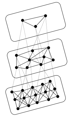
Hierarchical Navigable Small World
HNSW algorithm creates a multi-level graph to store vectors, enabling fast nearest neighbor searches by traversing connected nodes.
Algorithm
- Graph based approach: HNSW builds a multi-layered graph where each node represents a vector and edges are formed based on proximity. Higher layers contain fewer nodes and connect vectors that are further apart, while lower layers contain more nodes and connect vectors that are closer together.
- Search Process: The algorithm starts from the top layer of the graph, navigating down to lower layers progressively narrowing the search area. This allows for fast nearest neighbor retrieval.
Accuracy: HNSW is quite accurate and scales well for large datasets.
Use case: Ideal for high-dimensional data and large-scale applications where fast retrieval is important.
neighbours = 16  # Number of neighbors
index = faiss.IndexHNSWFlat(dimension, neighbours)
index.add(vectors)  # Add the vectors to the index
distances, indices = index.search(query, k)
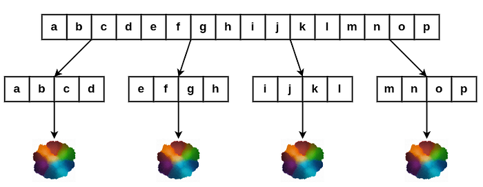
Product Quantization
Product Quantization reduces the memory usage by representing vectors as a combination of quantized components. It is often used when there is a need to store vectors compactly in memory and still perform fast similarity searches.
Algorithm
- Vector Quantization: PQ compresses high-dimensional vectors by dividing each vector into MM subvectors of lower dimensionality each of which is quantized separately. This reduces the dimensionality and makes it more efficient to store and search for vectors.
- Codebooks: Each sub-vector is treated as an individual vector and k-means clustering is used to generate the codebook for each sub-vector. The quantizer assigns each subvector to the closest centroid in its corresponding codebook. The combination of the indices of these centroids forms the compressed representation of the vector. The original vector x is now represented by the indices of the centroids in each codebook, which requires significantly less memory than storing the full high-dimensional vector. This compressed representation is much smaller, as you are only storing the index of the centroid for each sub-vector instead of the full sub-vector itself.
- Search: When querying, you also divide the query vector into the same number of sub-vectors and find the closest centroids from the codebooks. Once quantized, the search process involves comparing the quantized representations of vectors (which are indices) rather than the original high-dimensional vectors, making it faster.
Accuracy: PQ introduces some approximation errors due to quantization, but can be tuned to find a good balance between memory and accuracy.
Use case: Useful for very large datasets with constraints on memory usage.
sub_vectors = 16  # Number of subvectors
nbits = 8  # Number of bits per subvector
index = faiss.IndexPQ(dimension, sub_vectors, nbits)
index.train(vectors)  # Train the quantizer on the dataset
index.add(vectors)  # Add vectors to the index

# Searching the nearest neighbors
distances, indices = index.search(query, k)
Inverted File with Product Quantization
First the dataset is partitioned into clusters (as in IVF) and then each cluster is compressed using PQ.
Algorithm
- Cluster the Data (Inverted File): The result is an Inverted File Index, where each cluster corresponds to a bucket containing a set of vectors. This means that when querying, you only need to search a subset of the clusters rather than the entire dataset.
- Apply Product Quantization (PQ): Each vector is divided into sub-vectors (or blocks). These sub-vectors are independently quantized using separate codebooks (a set of centroids). Each codebook contains a set of centroids representing the possible values for that sub-vector. The vectors are then represented by indices pointing to the nearest centroid in the codebook for each sub-vector.
- Index Construction: The centroids of each cluster are stored, and each vector in the cluster is represented by the indices of the centroids of its sub-vectors.
- Search: The query vector is compared to the centroids of the clusters and the closest cluster/s are identified. The query vector is also divided into sub-vectors, and each sub-vector is quantized using the same codebooks that were used during indexing. The quantized representations of the query vector and the vectors in the clusters are compared to find the nearest neighbors.
Accuracy: The accuracy improves with a higher number of clusters and centroids per sub-vector, but this comes at the cost of increased memory usage and longer search times. Therefore, these parameters must be fine-tuned to strike a balance between speed and accuracy.
Use case: Ideal for large-scale high-dimensional vector search tasks where both speed and memory efficiency are essential.
nlist = 100  # Number of clusters
sub_vectors = 16  # Number of subvectors
nbits = 8  # Number of bits per subvector
quantizer = faiss.IndexFlatL2(dimension)  # The base quantizer
index = faiss.IndexIVFPQ(quantizer, dimension, nlist, sub_vectors, nbits)
index.train(vectors)  # Train the index
index.add(vectors)  # Add vectors to the index
Choosing the Right Index
- Small Dataset: If you have a small dataset of less than 100,000 vectors, using IndexFlatL2 or IndexFlatIP is often fine.
- Large Dataset: Consider using an IVF or HNSW index. IVF indexes are generally more memory efficient while HNSW is better for accuracy and fast retrieval.
- Memory constraints: If you’re constrained by memory but still need decent performance consider Product Quantization (PQ) or IVFPQ.
FAISS is designed to scale to billions of vectors, but choosing the right index and hardware is crucial for performance. Using faiss-gpu can significantly speed up both indexing and searching. If you’re using large-scale datasets or need real-time performance, you may benefit from enabling GPU-based FAISS.
Optimization Strategies
FAISS provides several methods for optimizing the performance of both index creation and query processing:
- Batch Searching: Instead of searching for one query vector at a time, FAISS supports batch searches. This allows multiple queries to be processed simultaneously, leveraging vectorized operations and parallelism on both CPUs and GPUs. By default FAISS uses multi-threading to utilize all available cores to parallelize the computation.
# Searching for multiple queries
query_batch = np.random.rand(10, dimension).astype('float32')  # 10 query vectors
D_batch, I_batch = index.search(query_batch, k)
- GPU Acceleration: FAISS provides GPU support for both index building and querying. If you’re working with extremely large datasets, leveraging GPU-accelerated search can lead to dramatic performance improvements.
# Using FAISS on GPU
res = faiss.StandardGpuResources()  # Initialize GPU resources
gpu_index = faiss.index_cpu_to_gpu(res, 0, index)  # Transfer index to GPU-0
D_gpu, I_gpu = gpu_index.search(query, k)
Conclusion
FAISS is a powerful tool for efficiently performing similarity search and clustering of high-dimensional data. By understanding the different types of indexes and optimization techniques, you can tailor the search process to suit the accuracy and performance requirements of your use case. Whether you’re working with large-scale image embeddings, document vectors or other machine learning models, FAISS provides a flexible and efficient solution to handle nearest neighbor search at scale.
By selecting the appropriate index type (Flat, IVF, PQ, HNSW) and utilizing the optimization strategies (batch search, GPU acceleration) you can significantly reduce the time and memory required for vector similarity search tasks while maintaining high accuracy.

 浙公网安备 33010602011771号