image similarity

背景

对于手写字体图片，检查手写于标准的相似度。

 

有三个要点：

• 首先度量指标是相似度
• 其次是图像的相似度
• 再次是手写字体图像的相似度

 

相似度度量

https://towardsdatascience.com/calculate-similarity-the-most-relevant-metrics-in-a-nutshell-9a43564f533e

两类度量方法：

1. 基于相似度度量
2. 基于距离的度量

Generally we can divide similarity metrics into two different groups:

1. Similarity Based Metrics:

• Pearson’s correlation
• Spearman’s correlation
• Kendall’s Tau
• Cosine similarity
• Jaccard similarity

2. Distance Based Metrics:

• Euclidean distance
• Manhattan distance

 

https://dataaspirant.com/five-most-popular-similarity-measures-implementation-in-python/

Table of contents

• Similarity
• Euclidean distance
  • Euclidean distance implementation in python
• Manhattan distance
  • Manhattan distance implementation in python
• Minkowski distance
  • Synonyms of Minkowski
  • Minkowski distance implementation in python
• Cosine Similarity
  • Cosine Similarity Implementation In Python
• Jaccard Similarity
  • Sets & Set Operations
  • Jaccard Similarity implementation in python
• Implementations of all five similarity measures implementation in python

 

图像相似度

https://stackoverflow.com/questions/11541154/checking-images-for-similarity-with-opencv

This is a huge topic, with answers from 3 lines of code to entire research magazines.

I will outline the most common such techniques and their results.

Comparing histograms

One of the simplest & fastest methods. Proposed decades ago as a means to find picture simmilarities. The idea is that a forest will have a lot of green, and a human face a lot of pink, or whatever. So, if you compare two pictures with forests, you'll get some simmilarity between histograms, because you have a lot of green in both.

Downside: it is too simplistic. A banana and a beach will look the same, as both are yellow.

OpenCV method: compareHist()

Template matching

A good example here matchTemplate finding good match. It convolves the search image with the one being search into. It is usually used to find smaller image parts in a bigger one.

Downsides: It only returns good results with identical images, same size & orientation.

OpenCV method: matchTemplate()

Feature matching

Considered one of the most efficient ways to do image search. A number of features are extracted from an image, in a way that guarantees the same features will be recognized again even when rotated, scaled or skewed. The features extracted this way can be matched against other image feature sets. Another image that has a high proportion of the features matching the first one is considered to be depicting the same scene.

Finding the homography between the two sets of points will allow you to also find the relative difference in shooting angle between the original pictures or the amount of overlapping.

There are a number of OpenCV tutorials/samples on this, and a nice video here. A whole OpenCV module (features2d) is dedicated to it.

Downsides: It may be slow. It is not perfect

 

 

SSIM

https://ourcodeworld.com/articles/read/991/how-to-calculate-the-structural-similarity-index-ssim-between-two-images-with-python

The Structural Similarity Index (SSIM) is a perceptual metric that quantifies the image quality degradation that is caused by processing such as data compression or by losses in data transmission. This metric is basically a full reference that requires 2 images from the same shot, this means 2 graphically identical images to the human eye. The second image generally is compressed or has a different quality, which is the goal of this index. SSIM is usually used in the video industry, but has as well a strong application in photography. SIM actually measures the perceptual difference between two similar images. It cannot judge which of the two is better: that must be inferred from knowing which is the original one and which has been exposed to additional processing such as compression or filters.

In this article, we will show you how to calculate this index between 2 images using Python.

 

# 3. Load the two input images
imageA = cv2.imread(args["first"])
imageB = cv2.imread(args["second"])

# 4. Convert the images to grayscale
grayA = cv2.cvtColor(imageA, cv2.COLOR_BGR2GRAY)
grayB = cv2.cvtColor(imageB, cv2.COLOR_BGR2GRAY)

# 5. Compute the Structural Similarity Index (SSIM) between the two
#    images, ensuring that the difference image is returned
(score, diff) = compare_ssim(grayA, grayB, full=True)
diff = (diff * 255).astype("uint8")

# 6. You can print only the score if you want
print("SSIM: {}".format(score))

 

Average Hash, pHash

http://www.hackerfactor.com/blog/index.php?/archives/432-Looks-Like-It.html

That's Perceptive!

Perceptual hash algorithms describe a class of comparable hash functions. Features in the image are used to generate a distinct (but not unique) fingerprint, and these fingerprints are comparable.

Perceptual hashes are a different concept compared to cryptographic hash functions like MD5 and SHA1. With cryptographic hashes, the hash values are random. The data used to generate the hash acts like a random seed, so the same data will generate the same result, but different data will create different results. Comparing two SHA1 hash values really only tells you two things. If the hashes are different, then the data is different. And if the hashes are the same, then the data is likely the same. (Since there is a possibility of a hash collision, having the same hash values does not guarantee the same data.) In contrast, perceptual hashes can be compared -- giving you a sense of similarity between the two data sets.

Every perceptual hash algorithm that I have come across has the same basic properties: images can be scaled larger or smaller, have different aspect ratios, and even minor coloring differences (contrast, brightness, etc.) and they will still match similar images. These are the same properties seen with TinEye. (But TinEye does appear to do more; I'll get to that in a moment.)

 

With pictures, high frequencies give you detail, while low frequencies show you structure. A large, detailed picture has lots of high frequencies. A very small picture lacks details, so it is all low frequencies. To show how the Average Hash algorithm works, I'll use a picture of my next wife, Alyson Hannigan.

1. Reduce size. The fastest way to remove high frequencies and detail is to shrink the image. In this case, shrink it to 8x8 so that there are 64 total pixels. Don't bother keeping the aspect ratio, just crush it down to fit an 8x8 square. This way, the hash will match any variation of the image, regardless of scale or aspect ratio.
   
2. Reduce color. The tiny 8x8 picture is converted to a grayscale. This changes the hash from 64 pixels (64 red, 64 green, and 64 blue) to 64 total colors.
   
3. Average the colors. Compute the mean value of the 64 colors.
   
4. Compute the bits. This is the fun part. Each bit is simply set based on whether the color value is above or below the mean.
   
5. Construct the hash. Set the 64 bits into a 64-bit integer. The order does not matter, just as long as you are consistent. (I set the bits from left to right, top to bottom using big-endian.)
   = = 8f373714acfcf4d0

The resulting hash won't change if the image is scaled or the aspect ratio changes. Increasing or decreasing the brightness or contrast, or even altering the colors won't dramatically change the hash value. And best of all: this is FAST!

 

imagehash

https://stackoverflow.com/questions/52736154/how-to-check-similarity-of-two-images-that-have-different-pixelization

You can use the imagehash library to compare similar images.

from PIL import Image
import imagehash
hash0 = imagehash.average_hash(Image.open('quora_photo.jpg')) 
hash1 = imagehash.average_hash(Image.open('twitter_photo.jpeg')) 
cutoff = 5

if hash0 - hash1 < cutoff:
  print('images are similar')
else:
  print('images are not similar')

Since the images are not exactly the same, there will be some differences. But imagehash will work even if the images are resized, compressed, different file formats or with adjusted contrast or colors.

The hash (or fingerprint, really) is derived from a 8x8 monochrome thumbnail of the image. But even with such a reduced sample, the similarity comparisons give quite accurate results. Adjust the cutoff to find a balance between false positives and false negatives that is acceptable.

 

 Histograms

https://opencv-python-tutroals.readthedocs.io/en/latest/py_tutorials/py_imgproc/py_histograms/py_histogram_begins/py_histogram_begins.html

So what is histogram ? You can consider histogram as a graph or plot, which gives you an overall idea about the intensity distribution of an image. It is a plot with pixel values (ranging from 0 to 255, not always) in X-axis and corresponding number of pixels in the image on Y-axis.

It is just another way of understanding the image. By looking at the histogram of an image, you get intuition about contrast, brightness, intensity distribution etc of that image. Almost all image processing tools today, provides features on histogram. Below is an image from Cambridge in Color website, and I recommend you to visit the site for more details.

You can see the image and its histogram. (Remember, this histogram is drawn for grayscale image, not color image). Left region of histogram shows the amount of darker pixels in image and right region shows the amount of brighter pixels. From the histogram, you can see dark region is more than brighter region, and amount of midtones (pixel values in mid-range, say around 127) are very less.

https://medium.com/de-bijenkorf-techblog/image-vector-representations-an-overview-of-ways-to-search-visually-similar-images-3f5729e72d07

disadvantages:

• although this solves the challenge nicely, the grabCut algorithm is not a fast function, which can be troublesome in a service that needs to do a fast (near real-time) calculation.
• The color histogram has very little descriptive power on shapes, and absolutely no clue on patterns within the colors. Because a striped blue shirt should not be matched to a plain blue shirt, This was also not a viable option for us.

 

 

image-similarity-measures

https://pypi.org/project/image-similarity-measures/

Implementation of eight evaluation metrics to access the similarity between two images. The eight metrics are as follows:

• Root mean square error (RMSE),
• Peak signal-to-noise ratio (PSNR),
• Structural Similarity Index (SSIM),
• Feature-based similarity index (FSIM),
• Information theoretic-based Statistic Similarity Measure (ISSM),
• Signal to reconstruction error ratio (SRE),
• Spectral angle mapper (SAM), and
• Universal image quality index (UIQ)

 

VGG16 for feature extraction

https://neurohive.io/en/popular-networks/vgg16/

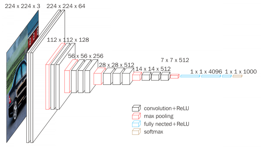
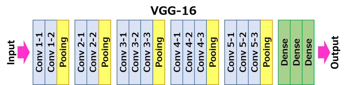
VGG16 – Convolutional Network for Classification and Detection

VGG16 is a convolutional neural network model proposed by K. Simonyan and A. Zisserman from the University of Oxford in the paper “Very Deep Convolutional Networks for Large-Scale Image Recognition”. The model achieves 92.7% top-5 test accuracy in ImageNet, which is a dataset of over 14 million images belonging to 1000 classes. It was one of the famous model submitted to ILSVRC-2014. It makes the improvement over AlexNet by replacing large kernel-sized filters (11 and 5 in the first and second convolutional layer, respectively) with multiple 3×3 kernel-sized filters one after another. VGG16 was trained for weeks and was using NVIDIA Titan Black GPU’s.

 

https://github.com/pappuyadav/image-similarity/blob/main/image_comaprision.ipynb

# Compare similarity between two images by using VGG16 as a feature extractor and cosine similarity as a distance metric
# Author: Pappu Kumar Yadav
from tensorflow.keras.applications.vgg16 import VGG16, preprocess_input
from tensorflow.keras.preprocessing.image import load_img, img_to_array
from tensorflow.keras.preprocessing import sequence
from tensorflow.keras.preprocessing import image
from tensorflow.keras.models import Model
from pickle import dump
import pickle
import matplotlib.pyplot as plt
from scipy import stats
from scipy import spatial
from scipy.stats import f_oneway

# load an image from file
image1 = load_img('/content/reference_image.jpg', target_size=(224, 224))
image2 = load_img('/content/compare_image.jpg', target_size=(224, 224))

# convert the image pixels to a numpy array
image1 = img_to_array(image1)
image2 = img_to_array(image2)
# reshape data for the VGG16 model
image1 = image1.reshape((1, image1.shape[0], image1.shape[1], image1.shape[2]))
image2 = image2.reshape((1, image2.shape[0], image2.shape[1], image2.shape[2]))
# prepare the image for the VGG16 model
image1 = preprocess_input(image1)
image2 = preprocess_input(image2)
# load model
model = VGG16()
# remove the output layer so as to use VGG16 as feature extractor and not as a classifier
model = Model(inputs=model.inputs, outputs=model.layers[-2].output)
# get extracted features
features1 = model.predict(image1)
features2 = model.predict(image2)
print(features1.shape)
print(features2.shape)


def image_similarity(vector1, vector2):
  result = 1 - spatial.distance.cosine(vector1, vector2)
  return result


fig, plot_num = plt.subplots(3)
plot_num[0].plot(features1[0])
plot_num[1].plot(features2[0])
plot_num[2].scatter(features1[0],features2[0])


aa=image_similarity(features1,features2)
print(aa)
bb=stats.pearsonr(features1[0],features2[0])
print(bb)


# save to file
dump(features1, open('features1.pkl', 'wb'))
dump(features2, open('features2.pkl', 'wb'))

with open('/content/features1.pkl', 'rb') as f:
  data1 = pickle.load(f)
with open('/content/features2.pkl', 'rb') as f:
  data2 = pickle.load(f)

with open("features1.txt", "wb") as abc:
  abc.write(data1)
with open("features2.txt", "wb") as abc:
  abc.write(data2)

 

计算两图的相似性

https://zhuanlan.zhihu.com/p/93893211

余弦相似度计算

哈希算法计算图片的相似度

直方图计算图片的相似度

SSIM（结构相似度度量）计算图片的相似度

基于互信息（Mutual Information）计算图片的相似度

 

• cosine相似度， 把图片像素展开为一个 向量，计算向量之间的夹角和模的算式， 得到了高维空间的一个统计值。 由于维度很高， 计算结果只是一个总体的量，不能反应局部差异性。
• 哈希算法， 类似于MD5之类， 可以用于查询相同图片。
• 直方图，是对颜色的分布进行统计， 计算颜色分布的相似性， 可以从色彩上找相似图片。
• SSIM, 用于评价照片压缩的质量。

 

手写字相似性(轮廓相似性)

与通用图片不同，字有鲜明的轮廓， 比较轮廓的相似性。

SIFT( Scale Invariant Feature Transform)

SIFT stands for Scale-Invariant Feature Transform and was first presented in 2004, by D.Lowe, University of British Columbia. SIFT is invariance to image scale and rotation. This algorithm is patented, so this algorithm is included in the Non-free module in OpenCV.

Major advantages of SIFT are

• Locality: features are local, so robust to occlusion and clutter (no prior segmentation)
• Distinctiveness: individual features can be matched to a large database of objects
• Quantity: many features can be generated for even small objects
• Efficiency: close to real-time performance
• Extensibility: can easily be extended to a wide range of different feature types, with each adding robustness

 

https://www.techgeekbuzz.com/sift-feature-extraction-using-opencv-in-python/

And if we talk about its features, everything in the image is the feature of the image. All the letters, Edges, Pyramids, objects, space between the letters, blobs, ridges, etc. are the features of the Image.

And to Detect these features from an image we use the Feature Detection Algorithms. There are various Features Detection Algorithms SIFT, SURF, GLOH, and HOG. But for this Python tutorial, we will be using SIFT Feature Extraction Algorithm using the OpenCV library and extract features in an Image.

 

 

 

import cv2 as cv

#load images
image1 = cv.imread("image1.jpg")
image2 = cv.imread("image2.jpg")

#convert to grayscale image
gray_scale1 = cv.cvtColor(image1, cv.COLOR_BGR2GRAY)
gray_scale2 = cv.cvtColor(image2, cv.COLOR_BGR2GRAY)

#initialize SIFT object
sift = cv.xfeatures2d.SIFT_create()

keypoints1, des1= sift.detectAndCompute(image1, None)
keypoints2, des2= sift.detectAndCompute(image2, None)

# initialize Brute force matching
bf = cv.BFMatcher(cv.NORM_L1, crossCheck=True)

matches = bf.match(des1,des2)

#sort the matches 
matches = sorted(matches, key= lambda match : match.distance)

matched_imge = cv.drawMatches(image1, keypoints1, image2, keypoints2, matches[:30], None)

cv.imshow("Matching Images", matched_imge)
cv.waitKey(0)

Output

 

 

https://medium.com/de-bijenkorf-techblog/image-vector-representations-an-overview-of-ways-to-search-visually-similar-images-3f5729e72d07

What SIFT and other algorithms are particularly good at is the recognition of patterns in images.

A big disadvantage is that these algorithms do not make use of color in combination with the patterns in the images. There is also something out there called colorSift, but so far we’ve not been able to get relevant results out of that. As color was a very important measure for us, we kept looking.

 

https://gist.github.com/duhaime/211365edaddf7ff89c0a36d9f3f7956c

import warnings
from skimage.measure import compare_ssim
from skimage.transform import resize
from scipy.stats import wasserstein_distance
from scipy.misc import imsave
from scipy.ndimage import imread
import numpy as np
import cv2

##
# Globals
##

warnings.filterwarnings('ignore')

# specify resized image sizes
height = 2**10
width = 2**10

##
# Functions
##

def get_img(path, norm_size=True, norm_exposure=False):
  '''
  Prepare an image for image processing tasks
  '''
  # flatten returns a 2d grayscale array
  img = imread(path, flatten=True).astype(int)
  # resizing returns float vals 0:255; convert to ints for downstream tasks
  if norm_size:
    img = resize(img, (height, width), anti_aliasing=True, preserve_range=True)
  if norm_exposure:
    img = normalize_exposure(img)
  return img


def get_histogram(img):
  '''
  Get the histogram of an image. For an 8-bit, grayscale image, the
  histogram will be a 256 unit vector in which the nth value indicates
  the percent of the pixels in the image with the given darkness level.
  The histogram's values sum to 1.
  '''
  h, w = img.shape
  hist = [0.0] * 256
  for i in range(h):
    for j in range(w):
      hist[img[i, j]] += 1
  return np.array(hist) / (h * w) 


def normalize_exposure(img):
  '''
  Normalize the exposure of an image.
  '''
  img = img.astype(int)
  hist = get_histogram(img)
  # get the sum of vals accumulated by each position in hist
  cdf = np.array([sum(hist[:i+1]) for i in range(len(hist))])
  # determine the normalization values for each unit of the cdf
  sk = np.uint8(255 * cdf)
  # normalize each position in the output image
  height, width = img.shape
  normalized = np.zeros_like(img)
  for i in range(0, height):
    for j in range(0, width):
      normalized[i, j] = sk[img[i, j]]
  return normalized.astype(int)


def earth_movers_distance(path_a, path_b):
  '''
  Measure the Earth Mover's distance between two images
  @args:
    {str} path_a: the path to an image file
    {str} path_b: the path to an image file
  @returns:
    TODO
  '''
  img_a = get_img(path_a, norm_exposure=True)
  img_b = get_img(path_b, norm_exposure=True)
  hist_a = get_histogram(img_a)
  hist_b = get_histogram(img_b)
  return wasserstein_distance(hist_a, hist_b)


def structural_sim(path_a, path_b):
  '''
  Measure the structural similarity between two images
  @args:
    {str} path_a: the path to an image file
    {str} path_b: the path to an image file
  @returns:
    {float} a float {-1:1} that measures structural similarity
      between the input images
  '''
  img_a = get_img(path_a)
  img_b = get_img(path_b)
  sim, diff = compare_ssim(img_a, img_b, full=True)
  return sim


def pixel_sim(path_a, path_b):
  '''
  Measure the pixel-level similarity between two images
  @args:
    {str} path_a: the path to an image file
    {str} path_b: the path to an image file
  @returns:
    {float} a float {-1:1} that measures structural similarity
      between the input images
  '''
  img_a = get_img(path_a, norm_exposure=True)
  img_b = get_img(path_b, norm_exposure=True)
  return np.sum(np.absolute(img_a - img_b)) / (height*width) / 255


def sift_sim(path_a, path_b):
  '''
  Use SIFT features to measure image similarity
  @args:
    {str} path_a: the path to an image file
    {str} path_b: the path to an image file
  @returns:
    TODO
  '''
  # initialize the sift feature detector
  orb = cv2.ORB_create()

  # get the images
  img_a = cv2.imread(path_a)
  img_b = cv2.imread(path_b)

  # find the keypoints and descriptors with SIFT
  kp_a, desc_a = orb.detectAndCompute(img_a, None)
  kp_b, desc_b = orb.detectAndCompute(img_b, None)

  # initialize the b
ruteforce matcher
  bf = cv2.BFMatcher(cv2.NORM_HAMMING, crossCheck=True)

  # match.distance is a float between {0:100} - lower means more similar
  matches = bf.match(desc_a, desc_b)
  similar_regions = [i for i in matches if i.distance < 70]
  if len(matches) == 0:
    return 0
  return len(similar_regions) / len(matches)


if __name__ == '__main__':
  img_a = 'a.jpg'
  img_b = 'b.jpg'
  # get the similarity values
  structural_sim = structural_sim(img_a, img_b)
  pixel_sim = pixel_sim(img_a, img_b)
  sift_sim = sift_sim(img_a, img_b)
  emd = earth_movers_distance(img_a, img_b)
  print(structural_sim, pixel_sim, sift_sim, emd)

 

SIFT字体书写相似性测试