Ensemble methods of sklearn

Ensemble methods

https://scikit-learn.org/stable/modules/ensemble.html

集成方法是组合几个基模型的预测，来改善单一模型的泛化性和 健壮性。

通常有两种集成方法：

（1）平均方法， 指导思想是， 独立训练介个模型， 平均化他们的预测。 这种方法， 减少变异。

装袋方法

随机森林方法

（2）提升方法， 基模型被依次训练， 一个努力去减少组合模型的偏差。 可以将几个弱模型组合为一个强大的模型。

AdaBoot

梯度提升法

The goal of ensemble methods is to combine the predictions of several base estimators built with a given learning algorithm in order to improve generalizability / robustness over a single estimator.

Two families of ensemble methods are usually distinguished:

• In averaging methods, the driving principle is to build several estimators independently and then to average their predictions. On average, the combined estimator is usually better than any of the single base estimator because its variance is reduced.

  Examples: Bagging methods, Forests of randomized trees, …

• By contrast, in boosting methods, base estimators are built sequentially and one tries to reduce the bias of the combined estimator. The motivation is to combine several weak models to produce a powerful ensemble.

  Examples: AdaBoost, Gradient Tree Boosting, …

 

Bagging meta-estimator

集成算法， 装袋法， 首先训练几个黑盒模型的， 在不同的原始训练集合的子集上， 然后聚集单个的预测，形成最终的预测。

In ensemble algorithms, bagging methods form a class of algorithms which build several instances of a black-box estimator on random subsets of the original training set and then aggregate their individual predictions to form a final prediction. These methods are used as a way to reduce the variance of a base estimator (e.g., a decision tree), by introducing randomization into its construction procedure and then making an ensemble out of it. In many cases, bagging methods constitute a very simple way to improve with respect to a single model, without making it necessary to adapt the underlying base algorithm. As they provide a way to reduce overfitting, bagging methods work best with strong and complex models (e.g., fully developed decision trees), in contrast with boosting methods which usually work best with weak models (e.g., shallow decision trees).

 

BaggingClassifier

https://scikit-learn.org/stable/modules/generated/sklearn.ensemble.BaggingClassifier.html#sklearn.ensemble.BaggingClassifier

A Bagging classifier.

A Bagging classifier is an ensemble meta-estimator that fits base classifiers each on random subsets of the original dataset and then aggregate their individual predictions (either by voting or by averaging) to form a final prediction. Such a meta-estimator can typically be used as a way to reduce the variance of a black-box estimator (e.g., a decision tree), by introducing randomization into its construction procedure and then making an ensemble out of it.

This algorithm encompasses several works from the literature. When random subsets of the dataset are drawn as random subsets of the samples, then this algorithm is known as Pasting [1]. If samples are drawn with replacement, then the method is known as Bagging [2]. When random subsets of the dataset are drawn as random subsets of the features, then the method is known as Random Subspaces [3]. Finally, when base estimators are built on subsets of both samples and features, then the method is known as Random Patches [4].

Read more in the User Guide.

>>> from sklearn.svm import SVC
>>> from sklearn.ensemble import BaggingClassifier
>>> from sklearn.datasets import make_classification
>>> X, y = make_classification(n_samples=100, n_features=4,
...                            n_informative=2, n_redundant=0,
...                            random_state=0, shuffle=False)
>>> clf = BaggingClassifier(base_estimator=SVC(),
...                         n_estimators=10, random_state=0).fit(X, y)
>>> clf.predict([[0, 0, 0, 0]])
array([1])

 

 

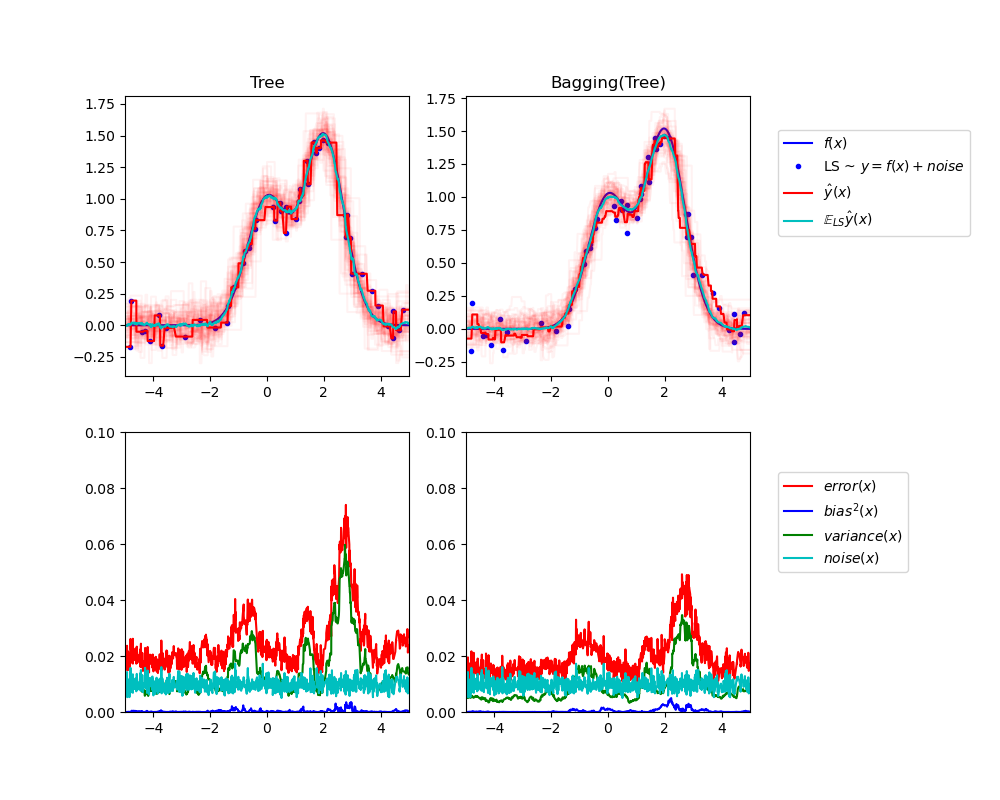
Single estimator versus bagging: bias-variance decomposition

比较偏差分解，对于单个模型和装袋法。

This example illustrates and compares the bias-variance decomposition of the expected mean squared error of a single estimator against a bagging ensemble.

 

print(__doc__)

# Author: Gilles Louppe <g.louppe@gmail.com>
# License: BSD 3 clause

import numpy as np
import matplotlib.pyplot as plt

from sklearn.ensemble import BaggingRegressor
from sklearn.tree import DecisionTreeRegressor

# Settings
n_repeat = 50       # Number of iterations for computing expectations
n_train = 50        # Size of the training set
n_test = 1000       # Size of the test set
noise = 0.1         # Standard deviation of the noise
np.random.seed(0)

# Change this for exploring the bias-variance decomposition of other
# estimators. This should work well for estimators with high variance (e.g.,
# decision trees or KNN), but poorly for estimators with low variance (e.g.,
# linear models).
estimators = [("Tree", DecisionTreeRegressor()),
              ("Bagging(Tree)", BaggingRegressor(DecisionTreeRegressor()))]

n_estimators = len(estimators)


# Generate data
def f(x):
    x = x.ravel()

    return np.exp(-x ** 2) + 1.5 * np.exp(-(x - 2) ** 2)


def generate(n_samples, noise, n_repeat=1):
    X = np.random.rand(n_samples) * 10 - 5
    X = np.sort(X)

    if n_repeat == 1:
        y = f(X) + np.random.normal(0.0, noise, n_samples)
    else:
        y = np.zeros((n_samples, n_repeat))

        for i in range(n_repeat):
            y[:, i] = f(X) + np.random.normal(0.0, noise, n_samples)

    X = X.reshape((n_samples, 1))

    return X, y


X_train = []
y_train = []

for i in range(n_repeat):
    X, y = generate(n_samples=n_train, noise=noise)
    X_train.append(X)
    y_train.append(y)

X_test, y_test = generate(n_samples=n_test, noise=noise, n_repeat=n_repeat)

plt.figure(figsize=(10, 8))

# Loop over estimators to compare
for n, (name, estimator) in enumerate(estimators):
    # Compute predictions
    y_predict = np.zeros((n_test, n_repeat))

    for i in range(n_repeat):
        estimator.fit(X_train[i], y_train[i])
        y_predict[:, i] = estimator.predict(X_test)

    # Bias^2 + Variance + Noise decomposition of the mean squared error
    y_error = np.zeros(n_test)

    for i in range(n_repeat):
        for j in range(n_repeat):
            y_error += (y_test[:, j] - y_predict[:, i]) ** 2

    y_error /= (n_repeat * n_repeat)

    y_noise = np.var(y_test, axis=1)
    y_bias = (f(X_test) - np.mean(y_predict, axis=1)) ** 2
    y_var = np.var(y_predict, axis=1)

    print("{0}: {1:.4f} (error) = {2:.4f} (bias^2) "
          " + {3:.4f} (var) + {4:.4f} (noise)".format(name,
                                                      np.mean(y_error),
                                                      np.mean(y_bias),
                                                      np.mean(y_var),
                                                      np.mean(y_noise)))

    # Plot figures
    plt.subplot(2, n_estimators, n + 1)
    plt.plot(X_test, f(X_test), "b", label="$f(x)$")
    plt.plot(X_train[0], y_train[0], ".b", label="LS ~ $y = f(x)+noise$")

    for i in range(n_repeat):
        if i == 0:
            plt.plot(X_test, y_predict[:, i], "r", label=r"$\^y(x)$")
        else:
            plt.plot(X_test, y_predict[:, i], "r", alpha=0.05)

    plt.plot(X_test, np.mean(y_predict, axis=1), "c",
             label=r"$\mathbb{E}_{LS} \^y(x)$")

    plt.xlim([-5, 5])
    plt.title(name)

    if n == n_estimators - 1:
        plt.legend(loc=(1.1, .5))

    plt.subplot(2, n_estimators, n_estimators + n + 1)
    plt.plot(X_test, y_error, "r", label="$error(x)$")
    plt.plot(X_test, y_bias, "b", label="$bias^2(x)$"),
    plt.plot(X_test, y_var, "g", label="$variance(x)$"),
    plt.plot(X_test, y_noise, "c", label="$noise(x)$")

    plt.xlim([-5, 5])
    plt.ylim([0, 0.1])

    if n == n_estimators - 1:

        plt.legend(loc=(1.1, .5))

plt.subplots_adjust(right=.75)
plt.show()

 

从图中可以看出，装袋法比单独模型，具有更大的稳定性。

Out:

Tree: 0.0255 (error) = 0.0003 (bias^2)  + 0.0152 (var) + 0.0098 (noise)
Bagging(Tree): 0.0196 (error) = 0.0004 (bias^2)  + 0.0092 (var) + 0.0098 (noise)

 

 

numpy.var

https://numpy.org/doc/stable/reference/generated/numpy.var.html#numpy.var

计算矩阵变异值， 实际上是均方差。

Compute the variance along the specified axis.

Returns the variance of the array elements, a measure of the spread of a distribution. The variance is computed for the flattened array by default, otherwise over the specified axis.

 

The variance is the average of the squared deviations from the mean, i.e., var = mean(x), where x = abs(a - a.mean())**2.

The mean is typically calculated as x.sum() / N, where N = len(x). If, however, ddof is specified, the divisor N - ddof is used instead. In standard statistical practice, ddof=1 provides an unbiased estimator of the variance of a hypothetical infinite population. ddof=0 provides a maximum likelihood estimate of the variance for normally distributed variables.

 

a = np.array([[1, 2], [3, 4]])

np.var(a)
1.25

np.var(a, axis=0)
array([1.,  1.])

np.var(a, axis=1)
array([0.25,  0.25])

 

Forests of randomized trees

集成学习模块，包括 两类平均算法， 基于随机决策树：

（1）RandomForest

（2）Extra-Trees

The sklearn.ensemble module includes two averaging algorithms based on randomized decision trees: the RandomForest algorithm and the Extra-Trees method. Both algorithms are perturb-and-combine techniques [B1998] specifically designed for trees. This means a diverse set of classifiers is created by introducing randomness in the classifier construction. The prediction of the ensemble is given as the averaged prediction of the individual classifiers.

As other classifiers, forest classifiers have to be fitted with two arrays: a sparse or dense array X of shape (n_samples, n_features) holding the training samples, and an array Y of shape (n_samples,) holding the target values (class labels) for the training samples:

 

>>> from sklearn.ensemble import RandomForestClassifier
>>> X = [[0, 0], [1, 1]]
>>> Y = [0, 1]
>>> clf = RandomForestClassifier(n_estimators=10)
>>> clf = clf.fit(X, Y)

 

Random Forests

随机森林中的 每一个树 是基于训练数据集中的抽样子集， 并且在训练分支的时候， 最好的分类是或者来自于全部的输入特征， 或者特征的随机子集。

随机数据

和

随机特征

这两个随机源， 保证的森林的变差可以减少， 不至于单个树的过拟合行为。

In random forests (see RandomForestClassifier and RandomForestRegressor classes), each tree in the ensemble is built from a sample drawn with replacement (i.e., a bootstrap sample) from the training set.

Furthermore, when splitting each node during the construction of a tree, the best split is found either from all input features or a random subset of size max_features. (See the parameter tuning guidelines for more details).

The purpose of these two sources of randomness is to decrease the variance of the forest estimator. Indeed, individual decision trees typically exhibit high variance and tend to overfit. The injected randomness in forests yield decision trees with somewhat decoupled prediction errors. By taking an average of those predictions, some errors can cancel out. Random forests achieve a reduced variance by combining diverse trees, sometimes at the cost of a slight increase in bias. In practice the variance reduction is often significant hence yielding an overall better model.

In contrast to the original publication [B2001], the scikit-learn implementation combines classifiers by averaging their probabilistic prediction, instead of letting each classifier vote for a single class.

 

Extremely Randomized Trees

极大化随机树， 在树进行分裂的过程中，随机方法被使用的跟进一步。

像随机森林， 随机的特征子集被使用， 但是不同的是， 随机森林寻找最大的区分阈值， 此方法多个阈值是被随机产生， 并且选择最好的一个阈值作为最终的分裂规则。

可以减少变异，但是增加偏置。

In extremely randomized trees (see ExtraTreesClassifier and ExtraTreesRegressor classes), randomness goes one step further in the way splits are computed. As in random forests, a random subset of candidate features is used, but instead of looking for the most discriminative thresholds, thresholds are drawn at random for each candidate feature and the best of these randomly-generated thresholds is picked as the splitting rule. This usually allows to reduce the variance of the model a bit more, at the expense of a slightly greater increase in bias:

 

>>> from sklearn.model_selection import cross_val_score
>>> from sklearn.datasets import make_blobs
>>> from sklearn.ensemble import RandomForestClassifier
>>> from sklearn.ensemble import ExtraTreesClassifier
>>> from sklearn.tree import DecisionTreeClassifier

>>> X, y = make_blobs(n_samples=10000, n_features=10, centers=100,
...     random_state=0)

>>> clf = DecisionTreeClassifier(max_depth=None, min_samples_split=2,
...     random_state=0)
>>> scores = cross_val_score(clf, X, y, cv=5)
>>> scores.mean()
0.98...

>>> clf = RandomForestClassifier(n_estimators=10, max_depth=None,
...     min_samples_split=2, random_state=0)
>>> scores = cross_val_score(clf, X, y, cv=5)
>>> scores.mean()
0.999...

>>> clf = ExtraTreesClassifier(n_estimators=10, max_depth=None,
...     min_samples_split=2, random_state=0)
>>> scores = cross_val_score(clf, X, y, cv=5)
>>> scores.mean() > 0.999
True

 

ExtraTreesClassifier

https://scikit-learn.org/stable/modules/generated/sklearn.ensemble.ExtraTreesClassifier.html#sklearn.ensemble.ExtraTreesClassifier

An extra-trees classifier.

This class implements a meta estimator that fits a number of randomized decision trees (a.k.a. extra-trees) on various sub-samples of the dataset and uses averaging to improve the predictive accuracy and control over-fitting.

 

>>> from sklearn.ensemble import ExtraTreesClassifier
>>> from sklearn.datasets import make_classification
>>> X, y = make_classification(n_features=4, random_state=0)
>>> clf = ExtraTreesClassifier(n_estimators=100, random_state=0)
>>> clf.fit(X, y)
ExtraTreesClassifier(random_state=0)
>>> clf.predict([[0, 0, 0, 0]])
array([1])

 

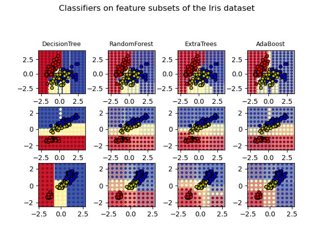
Plot the decision surfaces of ensembles of trees on the iris dataset

https://scikit-learn.org/stable/auto_examples/ensemble/plot_forest_iris.html#sphx-glr-auto-examples-ensemble-plot-forest-iris-py

比较四种模型在鸢尾花分类数据上的效果。

并绘制决策平面图。

 

Plot the decision surfaces of forests of randomized trees trained on pairs of features of the iris dataset.

This plot compares the decision surfaces learned by a decision tree classifier (first column), by a random forest classifier (second column), by an extra- trees classifier (third column) and by an AdaBoost classifier (fourth column).

In the first row, the classifiers are built using the sepal width and the sepal length features only, on the second row using the petal length and sepal length only, and on the third row using the petal width and the petal length only.

In descending order of quality, when trained (outside of this example) on all 4 features using 30 estimators and scored using 10 fold cross validation, we see:

ExtraTreesClassifier()  # 0.95 score
RandomForestClassifier()  # 0.94 score
AdaBoost(DecisionTree(max_depth=3))  # 0.94 score
DecisionTree(max_depth=None)  # 0.94 score

Increasing max_depth for AdaBoost lowers the standard deviation of the scores (but the average score does not improve).

See the console’s output for further details about each model.

In this example you might try to:

1. vary the max_depth for the DecisionTreeClassifier and AdaBoostClassifier, perhaps try max_depth=3 for the DecisionTreeClassifier or max_depth=None for AdaBoostClassifier

2. vary n_estimators

It is worth noting that RandomForests and ExtraTrees can be fitted in parallel on many cores as each tree is built independently of the others. AdaBoost’s samples are built sequentially and so do not use multiple cores.

 

print(__doc__)

import numpy as np
import matplotlib.pyplot as plt
from matplotlib.colors import ListedColormap

from sklearn.datasets import load_iris
from sklearn.ensemble import (RandomForestClassifier, ExtraTreesClassifier,
                              AdaBoostClassifier)
from sklearn.tree import DecisionTreeClassifier

# Parameters
n_classes = 3
n_estimators = 30
cmap = plt.cm.RdYlBu
plot_step = 0.02  # fine step width for decision surface contours
plot_step_coarser = 0.5  # step widths for coarse classifier guesses
RANDOM_SEED = 13  # fix the seed on each iteration

# Load data
iris = load_iris()

plot_idx = 1

models = [DecisionTreeClassifier(max_depth=None),
          RandomForestClassifier(n_estimators=n_estimators),
          ExtraTreesClassifier(n_estimators=n_estimators),
          AdaBoostClassifier(DecisionTreeClassifier(max_depth=3),
                             n_estimators=n_estimators)]

for pair in ([0, 1], [0, 2], [2, 3]):
    for model in models:
        # We only take the two corresponding features
        X = iris.data[:, pair]
        y = iris.target

        # Shuffle
        idx = np.arange(X.shape[0])
        np.random.seed(RANDOM_SEED)
        np.random.shuffle(idx)
        X = X[idx]
        y = y[idx]

        # Standardize
        mean = X.mean(axis=0)
        std = X.std(axis=0)
        X = (X - mean) / std

        # Train
        model.fit(X, y)

        scores = model.score(X, y)
        # Create a title for each column and the console by using str() and
        # slicing away useless parts of the string
        model_title = str(type(model)).split(
            ".")[-1][:-2][:-len("Classifier")]

        model_details = model_title
        if hasattr(model, "estimators_"):
            model_details += " with {} estimators".format(
                len(model.estimators_))
        print(model_details + " with features", pair,
              "has a score of", scores)

        plt.subplot(3, 4, plot_idx)
        if plot_idx <= len(models):
            # Add a title at the top of each column
            plt.title(model_title, fontsize=9)

        # Now plot the decision boundary using a fine mesh as input to a
        # filled contour plot
        x_min, x_max = X[:, 0].min() - 1, X[:, 0].max() + 1
        y_min, y_max = X[:, 1].min() - 1, X[:, 1].max() + 1
        xx, yy = np.meshgrid(np.arange(x_min, x_max, plot_step),
                             np.arange(y_min, y_max, plot_step))

        # Plot either a single DecisionTreeClassifier or alpha blend the
        # decision surfaces of the ensemble of classifiers
        if isinstance(model, DecisionTreeClassifier):
            Z = model.predict(np.c_[xx.ravel(), yy.ravel()])
            Z = Z.reshape(xx.shape)
            cs = plt.contourf(xx, yy, Z, cmap=cmap)
        else:
            # Choose alpha blend level with respect to the number
            # of estimators
            # that are in use (noting that AdaBoost can use fewer estimators
            # than its maximum if it achieves a good enough fit early on)
            estimator_alpha = 1.0 / len(model.estimators_)
            for tree in model.estimators_:
                Z = tree.predict(np.c_[xx.ravel(), yy.ravel()])
                Z = Z.reshape(xx.shape)
                cs = plt.contourf(xx, yy, Z, alpha=estimator_alpha, cmap=cmap)

        # Build a coarser grid to plot a set of ensemble classifications
        # to show how these are different to what we see in the decision
        # surfaces. These points are regularly space and do not have a
        # black outline
        xx_coarser, yy_coarser = np.meshgrid(
            np.arange(x_min, x_max, plot_step_coarser),
            np.arange(y_min, y_max, plot_step_coarser))
        Z_points_coarser = model.predict(np.c_[xx_coarser.ravel(),
                                         yy_coarser.ravel()]
                                         ).reshape(xx_coarser.shape)
        cs_points = plt.scatter(xx_coarser, yy_coarser, s=15,
                                c=Z_points_coarser, cmap=cmap,
                                edgecolors="none")

        # Plot the training points, these are clustered together and have a
        # black outline
        plt.scatter(X[:, 0], X[:, 1], c=y,
                    cmap=ListedColormap(['r', 'y', 'b']),
                    edgecolor='k', s=20)
        plot_idx += 1  # move on to the next plot in sequence

plt.suptitle("Classifiers on feature subsets of the Iris dataset", fontsize=12)
plt.axis("tight")
plt.tight_layout(h_pad=0.2, w_pad=0.2, pad=2.5)
plt.show()

 

 

Out:

DecisionTree with features [0, 1] has a score of 0.9266666666666666
RandomForest with 30 estimators with features [0, 1] has a score of 0.9266666666666666
ExtraTrees with 30 estimators with features [0, 1] has a score of 0.9266666666666666
AdaBoost with 30 estimators with features [0, 1] has a score of 0.8533333333333334
DecisionTree with features [0, 2] has a score of 0.9933333333333333
RandomForest with 30 estimators with features [0, 2] has a score of 0.9933333333333333
ExtraTrees with 30 estimators with features [0, 2] has a score of 0.9933333333333333
AdaBoost with 30 estimators with features [0, 2] has a score of 0.9933333333333333
DecisionTree with features [2, 3] has a score of 0.9933333333333333
RandomForest with 30 estimators with features [2, 3] has a score of 0.9933333333333333
ExtraTrees with 30 estimators with features [2, 3] has a score of 0.9933333333333333
AdaBoost with 30 estimators with features [2, 3] has a score of 0.9933333333333333

 

 

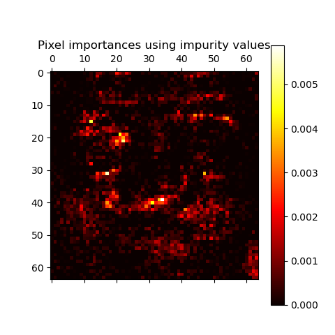
Pixel importances with a parallel forest of trees

https://scikit-learn.org/stable/auto_examples/ensemble/plot_forest_importances_faces.html#sphx-glr-auto-examples-ensemble-plot-forest-importances-faces-py

开启极大化树学习的并行模式

并绘制特征点的重要度图。

 

This example shows the use of forests of trees to evaluate the impurity-based importance of the pixels in an image classification task (faces). The hotter the pixel, the more important.

The code below also illustrates how the construction and the computation of the predictions can be parallelized within multiple jobs.

print(__doc__)

from time import time
import matplotlib.pyplot as plt

from sklearn.datasets import fetch_olivetti_faces
from sklearn.ensemble import ExtraTreesClassifier

# Number of cores to use to perform parallel fitting of the forest model
n_jobs = 1

# Load the faces dataset
data = fetch_olivetti_faces()
X, y = data.data, data.target

mask = y < 5  # Limit to 5 classes
X = X[mask]
y = y[mask]

# Build a forest and compute the pixel importances
print("Fitting ExtraTreesClassifier on faces data with %d cores..." % n_jobs)
t0 = time()
forest = ExtraTreesClassifier(n_estimators=1000,
                              max_features=128,
                              n_jobs=n_jobs,
                              random_state=0)

forest.fit(X, y)
print("done in %0.3fs" % (time() - t0))
importances = forest.feature_importances_
importances = importances.reshape(data.images[0].shape)

# Plot pixel importances
plt.matshow(importances, cmap=plt.cm.hot)
plt.title("Pixel importances with forests of trees")
plt.show()

 

 

Out:

Fitting ExtraTreesClassifier on faces data with 1 cores...
done in 2.008s

 

 

AdaBoost

集成模块包括了流行的提升算法 AdaBoost

此算法核心原理是 拟合一系列的弱学习者， 模型的表达能力很弱， 例如 小的决策树， 这些学习者在 重复修改的数据版本上学习。

所有模型的预测然后被通过 加权的投票， 来产生最终的预测。

 

The module sklearn.ensemble includes the popular boosting algorithm AdaBoost, introduced in 1995 by Freund and Schapire [FS1995].

The core principle of AdaBoost is to fit a sequence of weak learners (i.e., models that are only slightly better than random guessing, such as small decision trees) on repeatedly modified versions of the data. The predictions from all of them are then combined through a weighted majority vote (or sum) to produce the final prediction. The data modifications at each so-called boosting iteration consist of applying weights

, , …, to each of the training samples. Initially, those weights are all set to

, so that the first step simply trains a weak learner on the original data. For each successive iteration, the sample weights are individually modified and the learning algorithm is reapplied to the reweighted data. At a given step, those training examples that were incorrectly predicted by the boosted model induced at the previous step have their weights increased, whereas the weights are decreased for those that were predicted correctly. As iterations proceed, examples that are difficult to predict receive ever-increasing influence. Each subsequent weak learner is thereby forced to concentrate on the examples that are missed by the previous ones in the sequence [HTF].

AdaBoost can be used both for classification and regression problems:

• For multi-class classification, AdaBoostClassifier implements AdaBoost-SAMME and AdaBoost-SAMME.R [ZZRH2009].

• For regression, AdaBoostRegressor implements AdaBoost.R2 [D1997].

 

Discrete versus Real AdaBoost

https://scikit-learn.org/stable/auto_examples/ensemble/plot_adaboost_hastie_10_2.html#sphx-glr-auto-examples-ensemble-plot-adaboost-hastie-10-2-py

AdaBoost包括 离散提升算法 和 实数提升算法。

从图中看出， 实数提升算法，可以在较少的 模型数量上，快速收敛错误。尽管离散比实数差，但比单一模型效果都好。

 

This example is based on Figure 10.2 from Hastie et al 2009 1 and illustrates the difference in performance between the discrete SAMME 2 boosting algorithm and real SAMME.R boosting algorithm. Both algorithms are evaluated on a binary classification task where the target Y is a non-linear function of 10 input features.

Discrete SAMME AdaBoost adapts based on errors in predicted class labels whereas real SAMME.R uses the predicted class probabilities.

1

T. Hastie, R. Tibshirani and J. Friedman, “Elements of Statistical Learning Ed. 2”, Springer, 2009.

2

10. Zhu, H. Zou, S. Rosset, T. Hastie, “Multi-class AdaBoost”, 2009.

 

print(__doc__)

# Author: Peter Prettenhofer <peter.prettenhofer@gmail.com>,
#         Noel Dawe <noel.dawe@gmail.com>
#
# License: BSD 3 clause

import numpy as np
import matplotlib.pyplot as plt

from sklearn import datasets
from sklearn.tree import DecisionTreeClassifier
from sklearn.metrics import zero_one_loss
from sklearn.ensemble import AdaBoostClassifier


n_estimators = 400
# A learning rate of 1. may not be optimal for both SAMME and SAMME.R
learning_rate = 1.

X, y = datasets.make_hastie_10_2(n_samples=12000, random_state=1)

X_test, y_test = X[2000:], y[2000:]
X_train, y_train = X[:2000], y[:2000]

dt_stump = DecisionTreeClassifier(max_depth=1, min_samples_leaf=1)
dt_stump.fit(X_train, y_train)
dt_stump_err = 1.0 - dt_stump.score(X_test, y_test)

dt = DecisionTreeClassifier(max_depth=9, min_samples_leaf=1)
dt.fit(X_train, y_train)
dt_err = 1.0 - dt.score(X_test, y_test)

ada_discrete = AdaBoostClassifier(
    base_estimator=dt_stump,
    learning_rate=learning_rate,
    n_estimators=n_estimators,
    algorithm="SAMME")
ada_discrete.fit(X_train, y_train)

ada_real = AdaBoostClassifier(
    base_estimator=dt_stump,
    learning_rate=learning_rate,
    n_estimators=n_estimators,
    algorithm="SAMME.R")
ada_real.fit(X_train, y_train)

fig = plt.figure()
ax = fig.add_subplot(111)

ax.plot([1, n_estimators], [dt_stump_err] * 2, 'k-',
        label='Decision Stump Error')
ax.plot([1, n_estimators], [dt_err] * 2, 'k--',
        label='Decision Tree Error')

ada_discrete_err = np.zeros((n_estimators,))
for i, y_pred in enumerate(ada_discrete.staged_predict(X_test)):
    ada_discrete_err[i] = zero_one_loss(y_pred, y_test)

ada_discrete_err_train = np.zeros((n_estimators,))
for i, y_pred in enumerate(ada_discrete.staged_predict(X_train)):
    ada_discrete_err_train[i] = zero_one_loss(y_pred, y_train)

ada_real_err = np.zeros((n_estimators,))
for i, y_pred in enumerate(ada_real.staged_predict(X_test)):
    ada_real_err[i] = zero_one_loss(y_pred, y_test)

ada_real_err_train = np.zeros((n_estimators,))
for i, y_pred in enumerate(ada_real.staged_predict(X_train)):
    ada_real_err_train[i] = zero_one_loss(y_pred, y_train)

ax.plot(np.arange(n_estimators) + 1, ada_discrete_err,
        label='Discrete AdaBoost Test Error',
        color='red')
ax.plot(np.arange(n_estimators) + 1, ada_discrete_err_train,
        label='Discrete AdaBoost Train Error',
        color='blue')
ax.plot(np.arange(n_estimators) + 1, ada_real_err,
        label='Real AdaBoost Test Error',
        color='orange')
ax.plot(np.arange(n_estimators) + 1, ada_real_err_train,
        label='Real AdaBoost Train Error',
        color='green')

ax.set_ylim((0.0, 0.5))
ax.set_xlabel('n_estimators')
ax.set_ylabel('error rate')

leg = ax.legend(loc='upper right', fancybox=True)
leg.get_frame().set_alpha(0.7)

plt.show()

 

 

zero_one_loss

https://scikit-learn.org/stable/modules/generated/sklearn.metrics.zero_one_loss.html

 

Zero-one classification loss.

If normalize is True, return the fraction of misclassifications (float), else it returns the number of misclassifications (int). The best performance is 0.

 

>>> from sklearn.metrics import zero_one_loss
>>> y_pred = [1, 2, 3, 4]
>>> y_true = [2, 2, 3, 4]
>>> zero_one_loss(y_true, y_pred)
0.25
>>> zero_one_loss(y_true, y_pred, normalize=False)
1

 

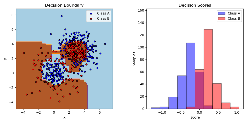
Two-class AdaBoost

https://scikit-learn.org/stable/auto_examples/ensemble/plot_adaboost_twoclass.html#sphx-glr-auto-examples-ensemble-plot-adaboost-twoclass-py

生成非线性可分问题，

使用 AdaBoost 和 深度为1的决策树拟合，

绘制决策平面和决策分数

This example fits an AdaBoosted decision stump on a non-linearly separable classification dataset composed of two “Gaussian quantiles” clusters (see sklearn.datasets.make_gaussian_quantiles) and plots the decision boundary and decision scores. The distributions of decision scores are shown separately for samples of class A and B. The predicted class label for each sample is determined by the sign of the decision score. Samples with decision scores greater than zero are classified as B, and are otherwise classified as A. The magnitude of a decision score determines the degree of likeness with the predicted class label. Additionally, a new dataset could be constructed containing a desired purity of class B, for example, by only selecting samples with a decision score above some value.

print(__doc__)

# Author: Noel Dawe <noel.dawe@gmail.com>
#
# License: BSD 3 clause

import numpy as np
import matplotlib.pyplot as plt

from sklearn.ensemble import AdaBoostClassifier
from sklearn.tree import DecisionTreeClassifier
from sklearn.datasets import make_gaussian_quantiles


# Construct dataset
X1, y1 = make_gaussian_quantiles(cov=2.,
                                 n_samples=200, n_features=2,
                                 n_classes=2, random_state=1)
X2, y2 = make_gaussian_quantiles(mean=(3, 3), cov=1.5,
                                 n_samples=300, n_features=2,
                                 n_classes=2, random_state=1)
X = np.concatenate((X1, X2))
y = np.concatenate((y1, - y2 + 1))

# Create and fit an AdaBoosted decision tree
bdt = AdaBoostClassifier(DecisionTreeClassifier(max_depth=1),
                         algorithm="SAMME",
                         n_estimators=200)

bdt.fit(X, y)

plot_colors = "br"
plot_step = 0.02
class_names = "AB"

plt.figure(figsize=(10, 5))

# Plot the decision boundaries
plt.subplot(121)
x_min, x_max = X[:, 0].min() - 1, X[:, 0].max() + 1
y_min, y_max = X[:, 1].min() - 1, X[:, 1].max() + 1
xx, yy = np.meshgrid(np.arange(x_min, x_max, plot_step),
                     np.arange(y_min, y_max, plot_step))

Z = bdt.predict(np.c_[xx.ravel(), yy.ravel()])
Z = Z.reshape(xx.shape)
cs = plt.contourf(xx, yy, Z, cmap=plt.cm.Paired)
plt.axis("tight")

# Plot the training points
for i, n, c in zip(range(2), class_names, plot_colors):
    idx = np.where(y == i)
    plt.scatter(X[idx, 0], X[idx, 1],
                c=c, cmap=plt.cm.Paired,
                s=20, edgecolor='k',
                label="Class %s" % n)
plt.xlim(x_min, x_max)
plt.ylim(y_min, y_max)
plt.legend(loc='upper right')
plt.xlabel('x')
plt.ylabel('y')
plt.title('Decision Boundary')

# Plot the two-class decision scores
twoclass_output = bdt.decision_function(X)
plot_range = (twoclass_output.min(), twoclass_output.max())
plt.subplot(122)
for i, n, c in zip(range(2), class_names, plot_colors):
    plt.hist(twoclass_output[y == i],
             bins=10,
             range=plot_range,
             facecolor=c,
             label='Class %s' % n,
             alpha=.5,
             edgecolor='k')
x1, x2, y1, y2 = plt.axis()
plt.axis((x1, x2, y1, y2 * 1.2))
plt.legend(loc='upper right')
plt.ylabel('Samples')
plt.xlabel('Score')
plt.title('Decision Scores')

plt.tight_layout()
plt.subplots_adjust(wspace=0.35)
plt.show()

 

 

Decision Tree Regression with AdaBoost

https://scikit-learn.org/stable/auto_examples/ensemble/plot_adaboost_regression.html#sphx-glr-auto-examples-ensemble-plot-adaboost-regression-py

AdaBoostRegressor 集合 决策树回归。

A decision tree is boosted using the AdaBoost.R2 1 algorithm on a 1D sinusoidal dataset with a small amount of Gaussian noise. 299 boosts (300 decision trees) is compared with a single decision tree regressor. As the number of boosts is increased the regressor can fit more detail.

1

8. Drucker, “Improving Regressors using Boosting Techniques”, 1997.

 

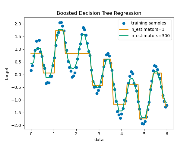
print(__doc__)

# Author: Noel Dawe <noel.dawe@gmail.com>
#
# License: BSD 3 clause

# importing necessary libraries
import numpy as np
import matplotlib.pyplot as plt
from sklearn.tree import DecisionTreeRegressor
from sklearn.ensemble import AdaBoostRegressor

# Create the dataset
rng = np.random.RandomState(1)
X = np.linspace(0, 6, 100)[:, np.newaxis]
y = np.sin(X).ravel() + np.sin(6 * X).ravel() + rng.normal(0, 0.1, X.shape[0])

# Fit regression model
regr_1 = DecisionTreeRegressor(max_depth=4)

regr_2 = AdaBoostRegressor(DecisionTreeRegressor(max_depth=4),
                          n_estimators=300, random_state=rng)

regr_1.fit(X, y)
regr_2.fit(X, y)

# Predict
y_1 = regr_1.predict(X)
y_2 = regr_2.predict(X)

# Plot the results
plt.figure()
plt.scatter(X, y, c="k", label="training samples")
plt.plot(X, y_1, c="g", label="n_estimators=1", linewidth=2)
plt.plot(X, y_2, c="r", label="n_estimators=300", linewidth=2)
plt.xlabel("data")
plt.ylabel("target")
plt.title("Boosted Decision Tree Regression")
plt.legend()
plt.show()

 

Gradient Tree Boosting

梯度提升决策树， 是是对任意可微损失函数的一种提升。

GBDT是一个精确的有效的 拿来就用 的 过程， 被用于回归和分类问题， 在广泛的领域， 包括 web搜索排名， 和生态学。

Gradient Tree Boosting or Gradient Boosted Decision Trees (GBDT) is a generalization of boosting to arbitrary differentiable loss functions. GBDT is an accurate and effective off-the-shelf procedure that can be used for both regression and classification problems in a variety of areas including Web search ranking and ecology.

The module sklearn.ensemble provides methods for both classification and regression via gradient boosted decision trees.

 

The usage and the parameters of GradientBoostingClassifier and GradientBoostingRegressor are described below. The 2 most important parameters of these estimators are n_estimators and learning_rate.

 

Gradient Boosting regression

https://scikit-learn.org/stable/auto_examples/ensemble/plot_gradient_boosting_regression.html#sphx-glr-auto-examples-ensemble-plot-gradient-boosting-regression-py

集成弱预测模型， 产生一个新的预测模型，

This example demonstrates Gradient Boosting to produce a predictive model from an ensemble of weak predictive models. Gradient boosting can be used for regression and classification problems. Here, we will train a model to tackle a diabetes regression task. We will obtain the results from GradientBoostingRegressor with least squares loss and 500 regression trees of depth 4.

Note: For larger datasets (n_samples >= 10000), please refer to HistGradientBoostingRegressor.

 

 

 

 

 

 

 

"""
============================
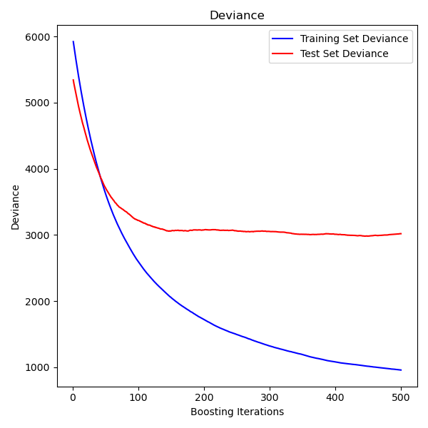
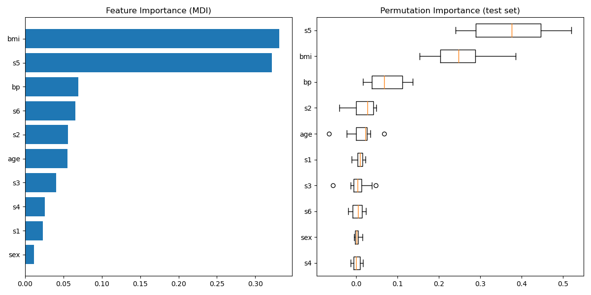
Gradient Boosting regression
============================

This example demonstrates Gradient Boosting to produce a predictive
model from an ensemble of weak predictive models. Gradient boosting can be used
for regression and classification problems. Here, we will train a model to
tackle a diabetes regression task. We will obtain the results from
:class:`~sklearn.ensemble.GradientBoostingRegressor` with least squares loss
and 500 regression trees of depth 4.

Note: For larger datasets (n_samples >= 10000), please refer to
:class:`~sklearn.ensemble.HistGradientBoostingRegressor`.
"""
print(__doc__)

# Author: Peter Prettenhofer <peter.prettenhofer@gmail.com>
#         Maria Telenczuk <https://github.com/maikia>
#         Katrina Ni <https://github.com/nilichen>
#
# License: BSD 3 clause

import matplotlib.pyplot as plt
import numpy as np
from sklearn import datasets, ensemble
from sklearn.inspection import permutation_importance
from sklearn.metrics import mean_squared_error
from sklearn.model_selection import train_test_split

# %%
# Load the data
# -------------------------------------
#
# First we need to load the data.

diabetes = datasets.load_diabetes()
X, y = diabetes.data, diabetes.target

# %%
# Data preprocessing
# -------------------------------------
#
# Next, we will split our dataset to use 90% for training and leave the rest
# for testing. We will also set the regression model parameters. You can play
# with these parameters to see how the results change.
#
# n_estimators : the number of boosting stages that will be performed.
# Later, we will plot deviance against boosting iterations.
#
# max_depth : limits the number of nodes in the tree.
# The best value depends on the interaction of the input variables.
#
# min_samples_split : the minimum number of samples required to split an
# internal node.
#
# learning_rate : how much the contribution of each tree will shrink.
#
# loss : loss function to optimize. The least squares function is  used in this
# case however, there are many other options (see
# :class:`~sklearn.ensemble.GradientBoostingRegressor` ).

X_train, X_test, y_train, y_test = train_test_split(
    X, y, test_size=0.1, random_state=13)

params = {'n_estimators': 500,
          'max_depth': 4,
          'min_samples_split': 5,
          'learning_rate': 0.01,
          'loss': 'ls'}

# %%
# Fit regression model
# -------------------------------------
#
# Now we will initiate the gradient boosting regressors and fit it with our
# training data. Let's also look and the mean squared error on the test data.

reg = ensemble.GradientBoostingRegressor(**params)
reg.fit(X_train, y_train)

mse = mean_squared_error(y_test, reg.predict(X_test))
print("The mean squared error (MSE) on test set: {:.4f}".format(mse))

# %%
# Plot training deviance
# -------------------------------------
#
# Finally, we will visualize the results. To do that we will first compute the
# test set deviance and then plot it against boosting iterations.

test_score = np.zeros((params['n_estimators'],), dtype=np.float64)
for i, y_pred in enumerate(reg.staged_predict(X_test)):
    test_score[i] = reg.loss_(y_test, y_pred)

fig = plt.figure(figsize=(6, 6))
plt.subplot(1, 1, 1)
plt.title('Deviance')
plt.plot(np.arange(params['n_estimators']) + 1, reg.train_score_, 'b-',
         label='Training Set Deviance')
plt.plot(np.arange(params['n_estimators']) + 1, test_score, 'r-',
         label='Test Set Deviance')
plt.legend(loc='upper right')
plt.xlabel('Boosting Iterations')
plt.ylabel('Deviance')
fig.tight_layout()
plt.show()

# %%
# Plot feature importance
# -------------------------------------
#
# Careful, impurity-based feature importances can be misleading for
# high cardinality features (many unique values). As an alternative,
# the permutation importances of ``reg`` can be computed on a
# held out test set. See :ref:`permutation_importance` for more details.
#
# For this example, the impurity-based and permutation methods identify the
# same 2 strongly predictive features but not in the same order. The third most
# predictive feature, "bp", is also the same for the 2 methods. The remaining
# features are less predictive and the error bars of the permutation plot
# show that they overlap with 0.

feature_importance = reg.feature_importances_
sorted_idx = np.argsort(feature_importance)
pos = np.arange(sorted_idx.shape[0]) + .5
fig = plt.figure(figsize=(12, 6))
plt.subplot(1, 2, 1)
plt.barh(pos, feature_importance[sorted_idx], align='center')
plt.yticks(pos, np.array(diabetes.feature_names)[sorted_idx])
plt.title('Feature Importance (MDI)')

result = permutation_importance(reg, X_test, y_test, n_repeats=10,
                                random_state=42, n_jobs=2)
sorted_idx = result.importances_mean.argsort()
plt.subplot(1, 2, 2)
plt.boxplot(result.importances[sorted_idx].T,
            vert=False, labels=np.array(diabetes.feature_names)[sorted_idx])
plt.title("Permutation Importance (test set)")
fig.tight_layout()
plt.show()

 

off-the-shelf

https://dictionary.cambridge.org/zhs/%E8%AF%8D%E5%85%B8/%E8%8B%B1%E8%AF%AD/off-the-shelf

立刻可用。

 

 

off-the-shelf 在英语中的意思

 

off-the-shelf

adjective [ before noun ]

uk

 

us

 

used to describe a product that is available immediately and does not need to be specially made to suit a particular purpose:

You can purchase off-the-shelf software or have it customized to suit your needs.

 

Voting Classifier

集成不同的子模型， 使用投票方法， 选举出预测结果。

The idea behind the VotingClassifier is to combine conceptually different machine learning classifiers and use a majority vote or the average predicted probabilities (soft vote) to predict the class labels. Such a classifier can be useful for a set of equally well performing model in order to balance out their individual weaknesses.

1.11.6.1. Majority Class Labels (Majority/Hard Voting)

In majority voting, the predicted class label for a particular sample is the class label that represents the majority (mode) of the class labels predicted by each individual classifier.

E.g., if the prediction for a given sample is

• classifier 1 -> class 1

• classifier 2 -> class 1

• classifier 3 -> class 2

the VotingClassifier (with voting='hard') would classify the sample as “class 1” based on the majority class label.

In the cases of a tie, the VotingClassifier will select the class based on the ascending sort order. E.g., in the following scenario

• classifier 1 -> class 2

• classifier 2 -> class 1

the class label 1 will be assigned to the sample.

 

 

>>> from sklearn import datasets
>>> from sklearn.model_selection import cross_val_score
>>> from sklearn.linear_model import LogisticRegression
>>> from sklearn.naive_bayes import GaussianNB
>>> from sklearn.ensemble import RandomForestClassifier
>>> from sklearn.ensemble import VotingClassifier

>>> iris = datasets.load_iris()
>>> X, y = iris.data[:, 1:3], iris.target

>>> clf1 = LogisticRegression(random_state=1)
>>> clf2 = RandomForestClassifier(n_estimators=50, random_state=1)
>>> clf3 = GaussianNB()

>>> eclf = VotingClassifier(
...     estimators=[('lr', clf1), ('rf', clf2), ('gnb', clf3)],
...     voting='hard')

>>> for clf, label in zip([clf1, clf2, clf3, eclf], ['Logistic Regression', 'Random Forest', 'naive Bayes', 'Ensemble']):
...     scores = cross_val_score(clf, X, y, scoring='accuracy', cv=5)
...     print("Accuracy: %0.2f (+/- %0.2f) [%s]" % (scores.mean(), scores.std(), label))
Accuracy: 0.95 (+/- 0.04) [Logistic Regression]
Accuracy: 0.94 (+/- 0.04) [Random Forest]
Accuracy: 0.91 (+/- 0.04) [naive Bayes]
Accuracy: 0.95 (+/- 0.04) [Ensemble]

 

1.11.6.3. Weighted Average Probabilities (Soft Voting)

In contrast to majority voting (hard voting), soft voting returns the class label as argmax of the sum of predicted probabilities.

Specific weights can be assigned to each classifier via the weights parameter. When weights are provided, the predicted class probabilities for each classifier are collected, multiplied by the classifier weight, and averaged. The final class label is then derived from the class label with the highest average probability.

To illustrate this with a simple example, let’s assume we have 3 classifiers and a 3-class classification problems where we assign equal weights to all classifiers: w1=1, w2=1, w3=1.

The weighted average probabilities for a sample would then be calculated as follows:

classifier	class 1	class 2	class 3
classifier 1	w1 * 0.2	w1 * 0.5	w1 * 0.3
classifier 2	w2 * 0.6	w2 * 0.3	w2 * 0.1
classifier 3	w3 * 0.3	w3 * 0.4	w3 * 0.3
weighted average	0.37	0.4	0.23

Here, the predicted class label is 2, since it has the highest average probability.

The following example illustrates how the decision regions may change when a soft VotingClassifier is used based on an linear Support Vector Machine, a Decision Tree, and a K-nearest neighbor classifier:

 

>>> from sklearn import datasets
>>> from sklearn.tree import DecisionTreeClassifier
>>> from sklearn.neighbors import KNeighborsClassifier
>>> from sklearn.svm import SVC
>>> from itertools import product
>>> from sklearn.ensemble import VotingClassifier

>>> # Loading some example data
>>> iris = datasets.load_iris()
>>> X = iris.data[:, [0, 2]]
>>> y = iris.target

>>> # Training classifiers
>>> clf1 = DecisionTreeClassifier(max_depth=4)
>>> clf2 = KNeighborsClassifier(n_neighbors=7)
>>> clf3 = SVC(kernel='rbf', probability=True)
>>> eclf = VotingClassifier(estimators=[('dt', clf1), ('knn', clf2), ('svc', clf3)],
...                         voting='soft', weights=[2, 1, 2])

>>> clf1 = clf1.fit(X, y)
>>> clf2 = clf2.fit(X, y)
>>> clf3 = clf3.fit(X, y)
>>> eclf = eclf.fit(X, y)

 

Voting Regressor

投票回归组合不同的回归模型， 返回平均预测值。

The idea behind the VotingRegressor is to combine conceptually different machine learning regressors and return the average predicted values. Such a regressor can be useful for a set of equally well performing models in order to balance out their individual weaknesses.

 

>>> from sklearn.datasets import load_diabetes
>>> from sklearn.ensemble import GradientBoostingRegressor
>>> from sklearn.ensemble import RandomForestRegressor
>>> from sklearn.linear_model import LinearRegression
>>> from sklearn.ensemble import VotingRegressor

>>> # Loading some example data
>>> X, y = load_diabetes(return_X_y=True)

>>> # Training classifiers
>>> reg1 = GradientBoostingRegressor(random_state=1)
>>> reg2 = RandomForestRegressor(random_state=1)
>>> reg3 = LinearRegression()
>>> ereg = VotingRegressor(estimators=[('gb', reg1), ('rf', reg2), ('lr', reg3)])
>>> ereg = ereg.fit(X, y)

 

 

Plot individual and voting regression predictions

https://scikit-learn.org/stable/auto_examples/ensemble/plot_voting_regressor.html#sphx-glr-auto-examples-ensemble-plot-voting-regressor-py

 

A voting regressor is an ensemble meta-estimator that fits several base regressors, each on the whole dataset. Then it averages the individual predictions to form a final prediction. We will use three different regressors to predict the data: GradientBoostingRegressor, RandomForestRegressor, and LinearRegression). Then the above 3 regressors will be used for the VotingRegressor.

Finally, we will plot the predictions made by all models for comparison.

We will work with the diabetes dataset which consists of 10 features collected from a cohort of diabetes patients. The target is a quantitative measure of disease progression one year after baseline.

"""
=================================================
Plot individual and voting regression predictions
=================================================

.. currentmodule:: sklearn

A voting regressor is an ensemble meta-estimator that fits several base
regressors, each on the whole dataset. Then it averages the individual
predictions to form a final prediction.
We will use three different regressors to predict the data:
:class:`~ensemble.GradientBoostingRegressor`,
:class:`~ensemble.RandomForestRegressor`, and
:class:`~linear_model.LinearRegression`).
Then the above 3 regressors will be used for the
:class:`~ensemble.VotingRegressor`.

Finally, we will plot the predictions made by all models for comparison.

We will work with the diabetes dataset which consists of 10 features
collected from a cohort of diabetes patients. The target is a quantitative
measure of disease progression one year after baseline.

"""
print(__doc__)

import matplotlib.pyplot as plt

from sklearn.datasets import load_diabetes
from sklearn.ensemble import GradientBoostingRegressor
from sklearn.ensemble import RandomForestRegressor
from sklearn.linear_model import LinearRegression
from sklearn.ensemble import VotingRegressor

# %%
# Training classifiers
# --------------------------------
#
# First, we will load the diabetes dataset and initiate a gradient boosting
# regressor, a random forest regressor and a linear regression. Next, we will
# use the 3 regressors to build the voting regressor:

X, y = load_diabetes(return_X_y=True)

# Train classifiers
reg1 = GradientBoostingRegressor(random_state=1)
reg2 = RandomForestRegressor(random_state=1)
reg3 = LinearRegression()

reg1.fit(X, y)
reg2.fit(X, y)
reg3.fit(X, y)

ereg = VotingRegressor([('gb', reg1), ('rf', reg2), ('lr', reg3)])
ereg.fit(X, y)

# %%
# Making predictions
# --------------------------------
#
# Now we will use each of the regressors to make the 20 first predictions.

xt = X[:20]

pred1 = reg1.predict(xt)
pred2 = reg2.predict(xt)
pred3 = reg3.predict(xt)
pred4 = ereg.predict(xt)

# %%
# Plot the results
# --------------------------------
#
# Finally, we will visualize the 20 predictions. The red stars show the average
# prediction made by :class:`~ensemble.VotingRegressor`.

plt.figure()
plt.plot(pred1, 'gd', label='GradientBoostingRegressor')
plt.plot(pred2, 'b^', label='RandomForestRegressor')
plt.plot(pred3, 'ys', label='LinearRegression')
plt.plot(pred4, 'r*', ms=10, label='VotingRegressor')

plt.tick_params(axis='x', which='both', bottom=False, top=False,
                labelbottom=False)
plt.ylabel('predicted')
plt.xlabel('training samples')
plt.legend(loc="best")
plt.title('Regressor predictions and their average')

plt.show()

 

StackingClassifier

https://scikit-learn.org/stable/modules/generated/sklearn.ensemble.StackingClassifier.html#sklearn.ensemble.StackingClassifier

将预测结果， 送入到另一个模型， 进行预测最终结果。

Stack of estimators with a final classifier.

Stacked generalization consists in stacking the output of individual estimator and use a classifier to compute the final prediction. Stacking allows to use the strength of each individual estimator by using their output as input of a final estimator.

Note that estimators_ are fitted on the full X while final_estimator_ is trained using cross-validated predictions of the base estimators using cross_val_predict.

Read more in the User Guide.

 

from sklearn.datasets import load_iris
from sklearn.ensemble import RandomForestClassifier
from sklearn.svm import LinearSVC
from sklearn.linear_model import LogisticRegression
from sklearn.preprocessing import StandardScaler
from sklearn.pipeline import make_pipeline
from sklearn.ensemble import StackingClassifier
X, y = load_iris(return_X_y=True)
estimators = [
    ('rf', RandomForestClassifier(n_estimators=10, random_state=42)),
    ('svr', make_pipeline(StandardScaler(),
                          LinearSVC(random_state=42)))
]
clf = StackingClassifier(
    estimators=estimators, final_estimator=LogisticRegression()
)
from sklearn.model_selection import train_test_split
X_train, X_test, y_train, y_test = train_test_split(
    X, y, stratify=y, random_state=42
)
clf.fit(X_train, y_train).score(X_test, y_test)