Neural network models (supervised) of sklearn

Neural network models (supervised)

https://scikit-learn.org/stable/modules/neural_networks_supervised.html#

sklearn实现的神经网络不支持大规模机器学习应用。

因为其没有GPU支持。

Warning

This implementation is not intended for large-scale applications. In particular, scikit-learn offers no GPU support. For much faster, GPU-based implementations, as well as frameworks offering much more flexibility to build deep learning architectures, see Related Projects.

Multi-layer Perceptron

多层感知机是一种监督型学习算法， 通过在数据集合上训练，学习出一个映射函数， 从特征域到目标域。

给定特征和目标，它能学习出非线性的函数逼近，为了分类或者回归问题。

其不同于逻辑回归，不同点在于 介于输入层和输出层之间的部分， 存在一个或者更多的非线性层， 叫隐含层。

如果没有隐含层，则退化为 逻辑回归。

其也存在 系数 和 截距 参数。

 

优点：

学习非线性模型的能力

支持在线学习

 

缺点：

存在多个局部极小点

需要调节大量超参

对特征伸缩敏感

The advantages of Multi-layer Perceptron are:

• Capability to learn non-linear models.

• Capability to learn models in real-time (on-line learning) using partial_fit.

The disadvantages of Multi-layer Perceptron (MLP) include:

• MLP with hidden layers have a non-convex loss function where there exists more than one local minimum. Therefore different random weight initializations can lead to different validation accuracy.

• MLP requires tuning a number of hyperparameters such as the number of hidden neurons, layers, and iterations.

• MLP is sensitive to feature scaling.

 

Classification

多层感知机算法使用反向传播方法。

支持输出分类预测概率。

Class MLPClassifier implements a multi-layer perceptron (MLP) algorithm that trains using Backpropagation.

MLP trains on two arrays: array X of size (n_samples, n_features), which holds the training samples represented as floating point feature vectors; and array y of size (n_samples,), which holds the target values (class labels) for the training samples:

>>>

>>> from sklearn.neural_network import MLPClassifier
>>> X = [[0., 0.], [1., 1.]]
>>> y = [0, 1]
>>> clf = MLPClassifier(solver='lbfgs', alpha=1e-5,
...                     hidden_layer_sizes=(5, 2), random_state=1)
...
>>> clf.fit(X, y)
MLPClassifier(alpha=1e-05, hidden_layer_sizes=(5, 2), random_state=1,
              solver='lbfgs')

After fitting (training), the model can predict labels for new samples:

>>>

>>> clf.predict([[2., 2.], [-1., -2.]])
array([1, 0])

MLP can fit a non-linear model to the training data. clf.coefs_ contains the weight matrices that constitute the model parameters:

>>>

>>> [coef.shape for coef in clf.coefs_]
[(2, 5), (5, 2), (2, 1)]

Currently, MLPClassifier supports only the Cross-Entropy loss function, which allows probability estimates by running the predict_proba method.

MLP trains using Backpropagation. More precisely, it trains using some form of gradient descent and the gradients are calculated using Backpropagation. For classification, it minimizes the Cross-Entropy loss function, giving a vector of probability estimates

per sample

:

>>>

>>> clf.predict_proba([[2., 2.], [1., 2.]])
array([[1.967...e-04, 9.998...-01],
       [1.967...e-04, 9.998...-01]])

 

 

支持多类别分类。

也支持多标签分类。

MLPClassifier supports multi-class classification by applying Softmax as the output function.

Further, the model supports multi-label classification in which a sample can belong to more than one class. For each class, the raw output passes through the logistic function. Values larger or equal to 0.5 are rounded to 1, otherwise to 0. For a predicted output of a sample, the indices where the value is 1 represents the assigned classes of that sample:

>>>

>>> X = [[0., 0.], [1., 1.]]
>>> y = [[0, 1], [1, 1]]
>>> clf = MLPClassifier(solver='lbfgs', alpha=1e-5,
...                     hidden_layer_sizes=(15,), random_state=1)
...
>>> clf.fit(X, y)
MLPClassifier(alpha=1e-05, hidden_layer_sizes=(15,), random_state=1,
              solver='lbfgs')
>>> clf.predict([[1., 2.]])
array([[1, 1]])
>>> clf.predict([[0., 0.]])
array([[0, 1]])

See the examples below and the docstring of MLPClassifier.fit for further information.

 

Regression

多层感知机如果在输出层使用非激活函数， 则生成的模型支持回归。

使用均方误差作为损失函数， 输出的值是连续的。

回归模型也支持多输出回归。

Class MLPRegressor implements a multi-layer perceptron (MLP) that trains using backpropagation with no activation function in the output layer, which can also be seen as using the identity function as activation function. Therefore, it uses the square error as the loss function, and the output is a set of continuous values.

MLPRegressor also supports multi-output regression, in which a sample can have more than one target.

 

Regularization

两种模型使用 正则参数， 来避免模型过拟合， 通过惩罚带有大量级的权重。

惩罚的越是严重， 其行为越接近于线性模型。

Both MLPRegressor and MLPClassifier use parameter alpha for regularization (L2 regularization) term which helps in avoiding overfitting by penalizing weights with large magnitudes. Following plot displays varying decision function with value of alpha.

 

MLPClassifier

https://scikit-learn.org/stable/modules/generated/sklearn.neural_network.MLPClassifier.html#sklearn.neural_network.MLPClassifier

Multi-layer Perceptron classifier.

This model optimizes the log-loss function using LBFGS or stochastic gradient descent.

 

>>> from sklearn.neural_network import MLPClassifier
>>> from sklearn.datasets import make_classification
>>> from sklearn.model_selection import train_test_split
>>> X, y = make_classification(n_samples=100, random_state=1)
>>> X_train, X_test, y_train, y_test = train_test_split(X, y, stratify=y,
...                                                     random_state=1)
>>> clf = MLPClassifier(random_state=1, max_iter=300).fit(X_train, y_train)
>>> clf.predict_proba(X_test[:1])
array([[0.038..., 0.961...]])
>>> clf.predict(X_test[:5, :])
array([1, 0, 1, 0, 1])
>>> clf.score(X_test, y_test)
0.8...

 

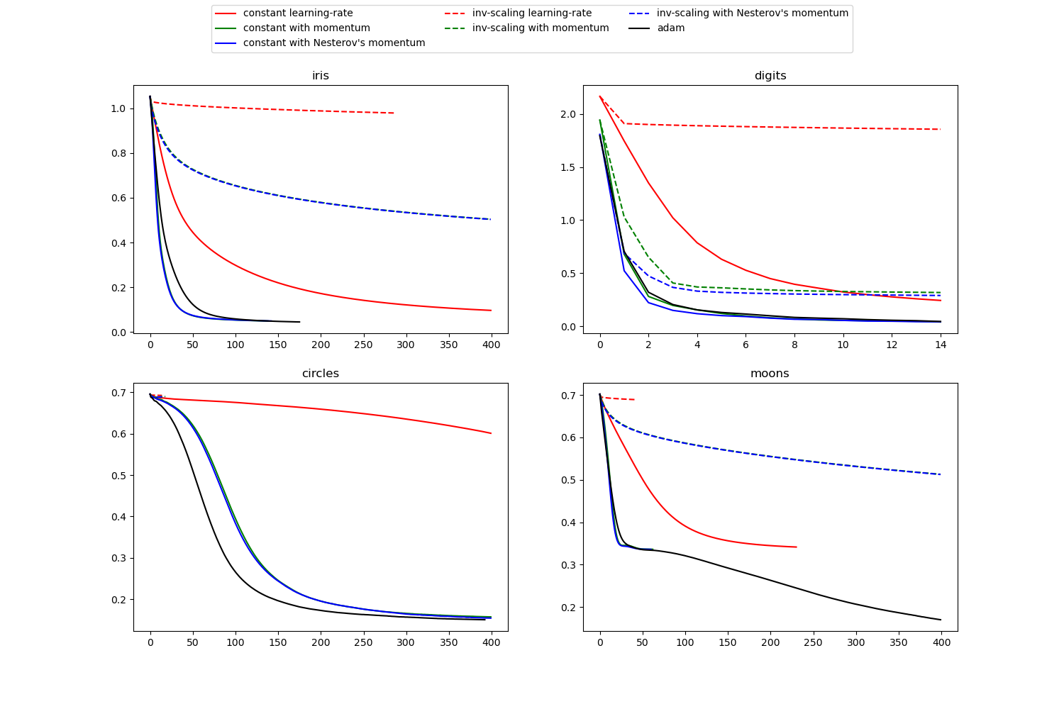
Compare Stochastic learning strategies for MLPClassifier

https://scikit-learn.org/stable/auto_examples/neural_networks/plot_mlp_training_curves.html#sphx-glr-auto-examples-neural-networks-plot-mlp-training-curves-py

对于不同的随机学习策略， 显示一些训练损失曲线。

This example visualizes some training loss curves for different stochastic learning strategies, including SGD and Adam. Because of time-constraints, we use several small datasets, for which L-BFGS might be more suitable. The general trend shown in these examples seems to carry over to larger datasets, however.

Note that those results can be highly dependent on the value of learning_rate_init.

 

 

print(__doc__)

import warnings

import matplotlib.pyplot as plt

from sklearn.neural_network import MLPClassifier
from sklearn.preprocessing import MinMaxScaler
from sklearn import datasets
from sklearn.exceptions import ConvergenceWarning

# different learning rate schedules and momentum parameters
params = [{'solver': 'sgd', 'learning_rate': 'constant', 'momentum': 0,
           'learning_rate_init': 0.2},
          {'solver': 'sgd', 'learning_rate': 'constant', 'momentum': .9,
           'nesterovs_momentum': False, 'learning_rate_init': 0.2},
          {'solver': 'sgd', 'learning_rate': 'constant', 'momentum': .9,
           'nesterovs_momentum': True, 'learning_rate_init': 0.2},
          {'solver': 'sgd', 'learning_rate': 'invscaling', 'momentum': 0,
           'learning_rate_init': 0.2},
          {'solver': 'sgd', 'learning_rate': 'invscaling', 'momentum': .9,
           'nesterovs_momentum': True, 'learning_rate_init': 0.2},
          {'solver': 'sgd', 'learning_rate': 'invscaling', 'momentum': .9,
           'nesterovs_momentum': False, 'learning_rate_init': 0.2},
          {'solver': 'adam', 'learning_rate_init': 0.01}]

labels = ["constant learning-rate", "constant with momentum",
          "constant with Nesterov's momentum",
          "inv-scaling learning-rate", "inv-scaling with momentum",
          "inv-scaling with Nesterov's momentum", "adam"]

plot_args = [{'c': 'red', 'linestyle': '-'},
             {'c': 'green', 'linestyle': '-'},
             {'c': 'blue', 'linestyle': '-'},
             {'c': 'red', 'linestyle': '--'},
             {'c': 'green', 'linestyle': '--'},
             {'c': 'blue', 'linestyle': '--'},
             {'c': 'black', 'linestyle': '-'}]


def plot_on_dataset(X, y, ax, name):
    # for each dataset, plot learning for each learning strategy
    print("\nlearning on dataset %s" % name)
    ax.set_title(name)

    X = MinMaxScaler().fit_transform(X)
    mlps = []
    if name == "digits":
        # digits is larger but converges fairly quickly
        max_iter = 15
    else:
        max_iter = 400

    for label, param in zip(labels, params):
        print("training: %s" % label)
        mlp = MLPClassifier(random_state=0,
                            max_iter=max_iter, **param)

        # some parameter combinations will not converge as can be seen on the
        # plots so they are ignored here
        with warnings.catch_warnings():
            warnings.filterwarnings("ignore", category=ConvergenceWarning,
                                    module="sklearn")
            mlp.fit(X, y)

        mlps.append(mlp)
        print("Training set score: %f" % mlp.score(X, y))
        print("Training set loss: %f" % mlp.loss_)
    for mlp, label, args in zip(mlps, labels, plot_args):
        ax.plot(mlp.loss_curve_, label=label, **args)


fig, axes = plt.subplots(2, 2, figsize=(15, 10))
# load / generate some toy datasets
iris = datasets.load_iris()
X_digits, y_digits = datasets.load_digits(return_X_y=True)
data_sets = [(iris.data, iris.target),
             (X_digits, y_digits),
             datasets.make_circles(noise=0.2, factor=0.5, random_state=1),
             datasets.make_moons(noise=0.3, random_state=0)]

for ax, data, name in zip(axes.ravel(), data_sets, ['iris', 'digits',
                                                    'circles', 'moons']):
    plot_on_dataset(*data, ax=ax, name=name)

fig.legend(ax.get_lines(), labels, ncol=3, loc="upper center")
plt.show()

 

Visualization of MLP weights on MNIST

https://scikit-learn.org/stable/auto_examples/neural_networks/plot_mnist_filters.html#sphx-glr-auto-examples-neural-networks-plot-mnist-filters-py

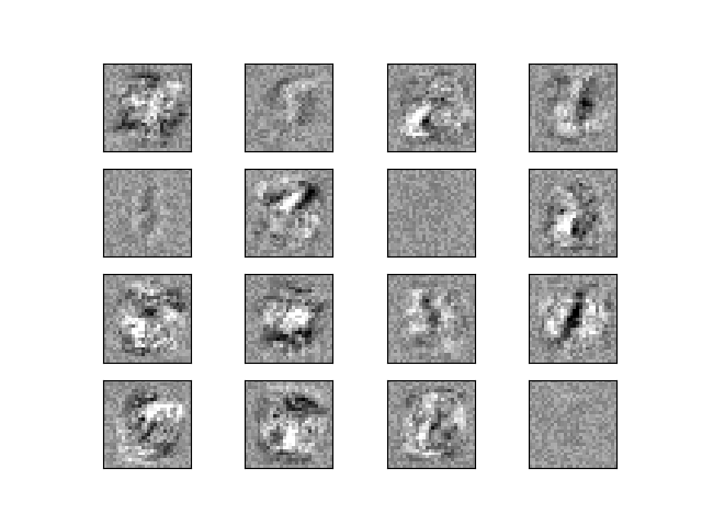
有时候观察学习系数，能提供学习行为的洞察。

例如如果权重看起来无结构的， 也许有些根本没有被使用，

或者如果存在非常大的系数， 表明正则化参数太小 或者 学习速率太高。

 

定义模型只有一个隐含层，在MNIST数据集合上训练模型， 对系数还原为图形。

 

从图中可以看出， 其中有三个 神经元 没有被使用。

Sometimes looking at the learned coefficients of a neural network can provide insight into the learning behavior. For example if weights look unstructured, maybe some were not used at all, or if very large coefficients exist, maybe regularization was too low or the learning rate too high.

This example shows how to plot some of the first layer weights in a MLPClassifier trained on the MNIST dataset.

The input data consists of 28x28 pixel handwritten digits, leading to 784 features in the dataset. Therefore the first layer weight matrix have the shape (784, hidden_layer_sizes[0]). We can therefore visualize a single column of the weight matrix as a 28x28 pixel image.

To make the example run faster, we use very few hidden units, and train only for a very short time. Training longer would result in weights with a much smoother spatial appearance. The example will throw a warning because it doesn’t converge, in this case this is what we want because of CI’s time constraints.

 

import warnings

import matplotlib.pyplot as plt
from sklearn.datasets import fetch_openml
from sklearn.exceptions import ConvergenceWarning
from sklearn.neural_network import MLPClassifier

print(__doc__)

# Load data from https://www.openml.org/d/554
X, y = fetch_openml('mnist_784', version=1, return_X_y=True)
X = X / 255.

# rescale the data, use the traditional train/test split
X_train, X_test = X[:60000], X[60000:]
y_train, y_test = y[:60000], y[60000:]

mlp = MLPClassifier(hidden_layer_sizes=(50,), max_iter=10, alpha=1e-4,
                    solver='sgd', verbose=10, random_state=1,
                    learning_rate_init=.1)

# this example won't converge because of CI's time constraints, so we catch the
# warning and are ignore it here
with warnings.catch_warnings():
    warnings.filterwarnings("ignore", category=ConvergenceWarning,
                            module="sklearn")
    mlp.fit(X_train, y_train)

print("Training set score: %f" % mlp.score(X_train, y_train))
print("Test set score: %f" % mlp.score(X_test, y_test))

fig, axes = plt.subplots(4, 4)
# use global min / max to ensure all weights are shown on the same scale
vmin, vmax = mlp.coefs_[0].min(), mlp.coefs_[0].max()
for coef, ax in zip(mlp.coefs_[0].T, axes.ravel()):
    ax.matshow(coef.reshape(28, 28), cmap=plt.cm.gray, vmin=.5 * vmin,
               vmax=.5 * vmax)
    ax.set_xticks(())
    ax.set_yticks(())

plt.show()

 

MLPRegressor

https://scikit-learn.org/stable/modules/generated/sklearn.neural_network.MLPRegressor.html#sklearn.neural_network.MLPRegressor

Multi-layer Perceptron regressor.

This model optimizes the squared-loss using LBFGS or stochastic gradient descent.

 

>>> from sklearn.neural_network import MLPRegressor
>>> from sklearn.datasets import make_regression
>>> from sklearn.model_selection import train_test_split
>>> X, y = make_regression(n_samples=200, random_state=1)
>>> X_train, X_test, y_train, y_test = train_test_split(X, y,
...                                                     random_state=1)
>>> regr = MLPRegressor(random_state=1, max_iter=500).fit(X_train, y_train)
>>> regr.predict(X_test[:2])
array([-0.9..., -7.1...])
>>> regr.score(X_test, y_test)
0.4...

 

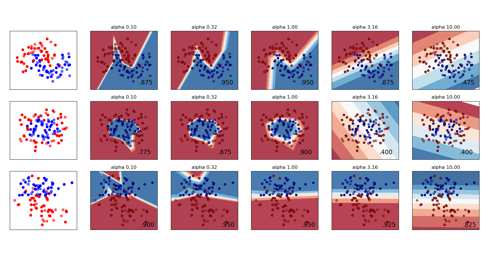
Varying regularization in Multi-layer Perceptron

https://scikit-learn.org/stable/auto_examples/neural_networks/plot_mlp_alpha.html#sphx-glr-auto-examples-neural-networks-plot-mlp-alpha-py

对于三种不同形状的数据集合， 调整 正则系数， 输出contour图， 查看分类平面效果。

A comparison of different values for regularization parameter ‘alpha’ on synthetic datasets. The plot shows that different alphas yield different decision functions.

Alpha is a parameter for regularization term, aka penalty term, that combats overfitting by constraining the size of the weights. Increasing alpha may fix high variance (a sign of overfitting) by encouraging smaller weights, resulting in a decision boundary plot that appears with lesser curvatures. Similarly, decreasing alpha may fix high bias (a sign of underfitting) by encouraging larger weights, potentially resulting in a more complicated decision boundary.

 

print(__doc__)


# Author: Issam H. Laradji
# License: BSD 3 clause

import numpy as np
from matplotlib import pyplot as plt
from matplotlib.colors import ListedColormap
from sklearn.model_selection import train_test_split
from sklearn.preprocessing import StandardScaler
from sklearn.datasets import make_moons, make_circles, make_classification
from sklearn.neural_network import MLPClassifier
from sklearn.pipeline import make_pipeline

h = .02  # step size in the mesh

alphas = np.logspace(-1, 1, 5)

classifiers = []
names = []
for alpha in alphas:
    classifiers.append(make_pipeline(
        StandardScaler(),
        MLPClassifier(
            solver='lbfgs', alpha=alpha, random_state=1, max_iter=2000,
            early_stopping=True, hidden_layer_sizes=[100, 100],
        )
    ))
    names.append(f"alpha {alpha:.2f}")

X, y = make_classification(n_features=2, n_redundant=0, n_informative=2,
                           random_state=0, n_clusters_per_class=1)
rng = np.random.RandomState(2)
X += 2 * rng.uniform(size=X.shape)
linearly_separable = (X, y)

datasets = [make_moons(noise=0.3, random_state=0),
            make_circles(noise=0.2, factor=0.5, random_state=1),
            linearly_separable]

figure = plt.figure(figsize=(17, 9))
i = 1
# iterate over datasets
for X, y in datasets:
    # split into training and test part
    X_train, X_test, y_train, y_test = train_test_split(X, y, test_size=.4)

    x_min, x_max = X[:, 0].min() - .5, X[:, 0].max() + .5
    y_min, y_max = X[:, 1].min() - .5, X[:, 1].max() + .5
    xx, yy = np.meshgrid(np.arange(x_min, x_max, h),
                         np.arange(y_min, y_max, h))

    # just plot the dataset first
    cm = plt.cm.RdBu
    cm_bright = ListedColormap(['#FF0000', '#0000FF'])
    ax = plt.subplot(len(datasets), len(classifiers) + 1, i)
    # Plot the training points
    ax.scatter(X_train[:, 0], X_train[:, 1], c=y_train, cmap=cm_bright)
    # and testing points
    ax.scatter(X_test[:, 0], X_test[:, 1], c=y_test, cmap=cm_bright, alpha=0.6)
    ax.set_xlim(xx.min(), xx.max())
    ax.set_ylim(yy.min(), yy.max())
    ax.set_xticks(())
    ax.set_yticks(())
    i += 1

    # iterate over classifiers
    for name, clf in zip(names, classifiers):
        ax = plt.subplot(len(datasets), len(classifiers) + 1, i)
        clf.fit(X_train, y_train)
        score = clf.score(X_test, y_test)

        # Plot the decision boundary. For that, we will assign a color to each
        # point in the mesh [x_min, x_max] x [y_min, y_max].
        if hasattr(clf, "decision_function"):
            Z = clf.decision_function(np.c_[xx.ravel(), yy.ravel()])
        else:
            Z = clf.predict_proba(np.c_[xx.ravel(), yy.ravel()])[:, 1]

        # Put the result into a color plot
        Z = Z.reshape(xx.shape)
        ax.contourf(xx, yy, Z, cmap=cm, alpha=.8)

        # Plot also the training points
        ax.scatter(X_train[:, 0], X_train[:, 1], c=y_train, cmap=cm_bright,
                   edgecolors='black', s=25)
        # and testing points
        ax.scatter(X_test[:, 0], X_test[:, 1], c=y_test, cmap=cm_bright,
                   alpha=0.6, edgecolors='black', s=25)

        ax.set_xlim(xx.min(), xx.max())
        ax.set_ylim(yy.min(), yy.max())
        ax.set_xticks(())
        ax.set_yticks(())
        ax.set_title(name)
        ax.text(xx.max() - .3, yy.min() + .3, ('%.2f' % score).lstrip('0'),
                size=15, horizontalalignment='right')
        i += 1

figure.subplots_adjust(left=.02, right=.98)
plt.show()