Support Vector Machines of sklearn

Support Vector Machines

https://scikit-learn.org/stable/modules/svm.html#

支持向量是监督学习方法的集合， 可以用于 分类 回归 和 异常检测。

优点:

在高维空间非常有效

仍然有效，当样本数目小于特征维度数目

不同于KNN， 在模型中只使用训练样本的子集， 内存上是高效的

多才的，使用不同的核函数用于决策函数

 

缺点：

如果特征的数目大于样本数据， 需要避免过拟合

SVM不提供概率估计，打分

Support vector machines (SVMs) are a set of supervised learning methods used for classification, regression and outliers detection.

The advantages of support vector machines are:

• Effective in high dimensional spaces.

• Still effective in cases where number of dimensions is greater than the number of samples.

• Uses a subset of training points in the decision function (called support vectors), so it is also memory efficient.

• Versatile: different Kernel functions can be specified for the decision function. Common kernels are provided, but it is also possible to specify custom kernels.

The disadvantages of support vector machines include:

• If the number of features is much greater than the number of samples, avoid over-fitting in choosing Kernel functions and regularization term is crucial.

• SVMs do not directly provide probability estimates, these are calculated using an expensive five-fold cross-validation (see Scores and probabilities, below).

The support vector machines in scikit-learn support both dense (numpy.ndarray and convertible to that by numpy.asarray) and sparse (any scipy.sparse) sample vectors as input. However, to use an SVM to make predictions for sparse data, it must have been fit on such data. For optimal performance, use C-ordered numpy.ndarray (dense) or scipy.sparse.csr_matrix (sparse) with dtype=float64.

 

Classification

三种SVC模型可以用于 二值分类 和 多类分类。

SVC 和 NuSVC 依赖不同的数学公式，有些许不同的参数。

LinearSVC 是另外一种支持向量实现， 其内置线性核。

SVC, NuSVC and LinearSVC are classes capable of performing binary and multi-class classification on a dataset.

SVC and NuSVC are similar methods, but accept slightly different sets of parameters and have different mathematical formulations (see section Mathematical formulation). On the other hand, LinearSVC is another (faster) implementation of Support Vector Classification for the case of a linear kernel. Note that LinearSVC does not accept parameter kernel, as this is assumed to be linear. It also lacks some of the attributes of SVC and NuSVC, like support_.

As other classifiers, SVC, NuSVC and LinearSVC take as input two arrays: an array X of shape (n_samples, n_features) holding the training samples, and an array y of class labels (strings or integers), of shape (n_samples):

 

使用方法

>>> from sklearn import svm
>>> X = [[0, 0], [1, 1]]
>>> y = [0, 1]
>>> clf = svm.SVC()
>>> clf.fit(X, y)
SVC()

After being fitted, the model can then be used to predict new values:

>>> clf.predict([[2., 2.]])
array([1])

 

SVM决策函数依赖于训练数据的一些子集， 这些数据被叫做支持向量。

信息存储于 support_vectors_, support_ and n_support_

SVMs decision function (detailed in the Mathematical formulation) depends on some subset of the training data, called the support vectors. Some properties of these support vectors can be found in attributes support_vectors_, support_ and n_support_:

>>> # get support vectors
>>> clf.support_vectors_
array([[0., 0.],
       [1., 1.]])
>>> # get indices of support vectors
>>> clf.support_
array([0, 1]...)
>>> # get number of support vectors for each class
>>> clf.n_support_
array([1, 1]...)

 

SVM: Maximum margin separating hyperplane

https://scikit-learn.org/stable/auto_examples/svm/plot_separating_hyperplane.html#sphx-glr-auto-examples-svm-plot-separating-hyperplane-py

对于二值可分的数据， 使用支持向量基，带有 线性核， 绘出 最大化的 边际可分平面。

对于样本空间， 使用meshgrid覆盖， 并将模型的决策函数应用于覆盖集合点， 获得决策值，

对于决策值 使用contour线绘出分割边际和中心线。

Plot the maximum margin separating hyperplane within a two-class separable dataset using a Support Vector Machine classifier with linear kernel.

 

print(__doc__)

import numpy as np
import matplotlib.pyplot as plt
from sklearn import svm
from sklearn.datasets import make_blobs


# we create 40 separable points
X, y = make_blobs(n_samples=40, centers=2, random_state=6)

# fit the model, don't regularize for illustration purposes
clf = svm.SVC(kernel='linear', C=1000)
clf.fit(X, y)

plt.scatter(X[:, 0], X[:, 1], c=y, s=30, cmap=plt.cm.Paired)

# plot the decision function
ax = plt.gca()
xlim = ax.get_xlim()
ylim = ax.get_ylim()

# create grid to evaluate model
xx = np.linspace(xlim[0], xlim[1], 30)
yy = np.linspace(ylim[0], ylim[1], 30)
YY, XX = np.meshgrid(yy, xx)
xy = np.vstack([XX.ravel(), YY.ravel()]).T
Z = clf.decision_function(xy).reshape(XX.shape)

# plot decision boundary and margins
ax.contour(XX, YY, Z, colors='k', levels=[-1, 0, 1], alpha=0.5,
           linestyles=['--', '-', '--'])
# plot support vectors
ax.scatter(clf.support_vectors_[:, 0], clf.support_vectors_[:, 1], s=100,
           linewidth=1, facecolors='none', edgecolors='k')
plt.show()

 

contour

https://ww2.mathworks.cn/help/matlab/ref/contour.html

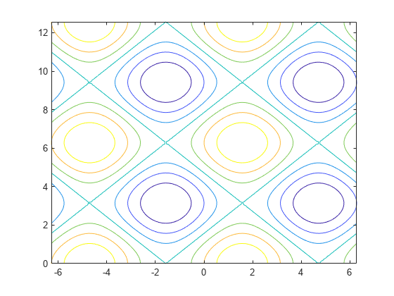
类似气象图中的等高线。

 

创建矩阵 X 和 Y，用于在 x-y 平面中定义一个网格。将矩阵 Z 定义为该网格上方的高度。然后绘制 Z 的等高线。

x = linspace(-2*pi,2*pi);
y = linspace(0,4*pi);
[X,Y] = meshgrid(x,y);
Z = sin(X)+cos(Y);
contour(X,Y,Z)

 

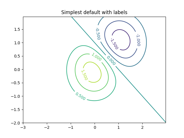
https://matplotlib.org/3.3.1/api/_as_gen/matplotlib.axes.Axes.contour.html

https://matplotlib.org/3.3.1/gallery/images_contours_and_fields/contour_demo.html#sphx-glr-gallery-images-contours-and-fields-contour-demo-py

import matplotlib
import numpy as np
import matplotlib.cm as cm
import matplotlib.pyplot as plt


delta = 0.025
x = np.arange(-3.0, 3.0, delta)
y = np.arange(-2.0, 2.0, delta)
X, Y = np.meshgrid(x, y)
Z1 = np.exp(-X**2 - Y**2)
Z2 = np.exp(-(X - 1)**2 - (Y - 1)**2)
Z = (Z1 - Z2) * 2

fig, ax = plt.subplots()
CS = ax.contour(X, Y, Z)
ax.clabel(CS, inline=True, fontsize=10)
ax.set_title('Simplest default with labels')

 

 

 

Non-linear SVM

https://scikit-learn.org/stable/auto_examples/svm/plot_svm_nonlinear.html#sphx-glr-auto-examples-svm-plot-svm-nonlinear-py

生成典型的 XOR 线性不可分的数据集合。

使用决策函数值，绘制颜色图和contour线。

Perform binary classification using non-linear SVC with RBF kernel. The target to predict is a XOR of the inputs.

The color map illustrates the decision function learned by the SVC.

 

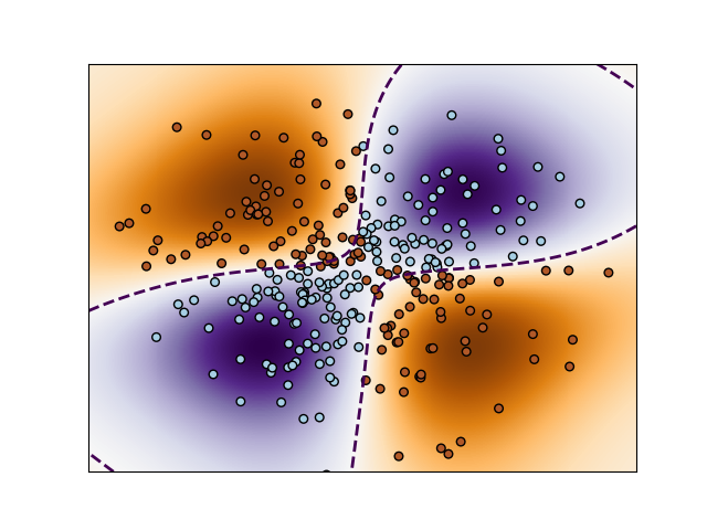
print(__doc__)

import numpy as np
import matplotlib.pyplot as plt
from sklearn import svm

xx, yy = np.meshgrid(np.linspace(-3, 3, 500),
                     np.linspace(-3, 3, 500))
np.random.seed(0)
X = np.random.randn(300, 2)
Y = np.logical_xor(X[:, 0] > 0, X[:, 1] > 0)

# fit the model
clf = svm.NuSVC(gamma='auto')
clf.fit(X, Y)

# plot the decision function for each datapoint on the grid
Z = clf.decision_function(np.c_[xx.ravel(), yy.ravel()])
Z = Z.reshape(xx.shape)

plt.imshow(Z, interpolation='nearest',
           extent=(xx.min(), xx.max(), yy.min(), yy.max()), aspect='auto',
           origin='lower', cmap=plt.cm.PuOr_r)
contours = plt.contour(xx, yy, Z, levels=[0], linewidths=2,
                       linestyles='dashed')
plt.scatter(X[:, 0], X[:, 1], s=30, c=Y, cmap=plt.cm.Paired,
            edgecolors='k')
plt.xticks(())
plt.yticks(())
plt.axis([-3, 3, -3, 3])
plt.show()

 

NuSVC

https://scikit-learn.org/stable/modules/generated/sklearn.svm.NuSVC.html#sklearn.svm.NuSVC

可以控制支持向量的数目。

Nu-Support Vector Classification.

Similar to SVC but uses a parameter to control the number of support vectors.

The implementation is based on libsvm.

>>> import numpy as np
>>> X = np.array([[-1, -1], [-2, -1], [1, 1], [2, 1]])
>>> y = np.array([1, 1, 2, 2])
>>> from sklearn.pipeline import make_pipeline
>>> from sklearn.preprocessing import StandardScaler
>>> from sklearn.svm import NuSVC
>>> clf = make_pipeline(StandardScaler(), NuSVC())
>>> clf.fit(X, y)
Pipeline(steps=[('standardscaler', StandardScaler()), ('nusvc', NuSVC())])
>>> print(clf.predict([[-0.8, -1]]))
[1]

 

SVM-Anova: SVM with univariate feature selection

https://scikit-learn.org/stable/auto_examples/svm/plot_svm_anova.html#sphx-glr-auto-examples-svm-plot-svm-anova-py

一个完整的 集成 特征选择 标准化 和 SVC模型的流水线。

确定特征选择的参数的最优值。

This example shows how to perform univariate feature selection before running a SVC (support vector classifier) to improve the classification scores. We use the iris dataset (4 features) and add 36 non-informative features. We can find that our model achieves best performance when we select around 10% of features.

 

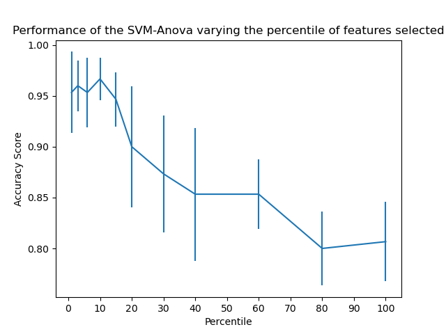
print(__doc__)

import numpy as np
import matplotlib.pyplot as plt
from sklearn.datasets import load_iris
from sklearn.feature_selection import SelectPercentile, chi2
from sklearn.model_selection import cross_val_score
from sklearn.pipeline import Pipeline
from sklearn.preprocessing import StandardScaler
from sklearn.svm import SVC


# #############################################################################
# Import some data to play with
X, y = load_iris(return_X_y=True)
# Add non-informative features
np.random.seed(0)
X = np.hstack((X, 2 * np.random.random((X.shape[0], 36))))

# #############################################################################
# Create a feature-selection transform, a scaler and an instance of SVM that we
# combine together to have an full-blown estimator
clf = Pipeline([('anova', SelectPercentile(chi2)),
                ('scaler', StandardScaler()),
                ('svc', SVC(gamma="auto"))])

# #############################################################################
# Plot the cross-validation score as a function of percentile of features
score_means = list()
score_stds = list()
percentiles = (1, 3, 6, 10, 15, 20, 30, 40, 60, 80, 100)

for percentile in percentiles:
    clf.set_params(anova__percentile=percentile)
    this_scores = cross_val_score(clf, X, y)
    score_means.append(this_scores.mean())
    score_stds.append(this_scores.std())

plt.errorbar(percentiles, score_means, np.array(score_stds))
plt.title(
    'Performance of the SVM-Anova varying the percentile of features selected')
plt.xticks(np.linspace(0, 100, 11, endpoint=True))
plt.xlabel('Percentile')
plt.ylabel('Accuracy Score')
plt.axis('tight')
plt.show()

 

Multi-class classification

SVC 和 NuSVC 对于多分类问题， 采用 一对一的策略， 总共需要 n_classes * (n_classes - 1) / 2 个模型， 用于区分两个类别。

SVC and NuSVC implement the “one-versus-one” approach for multi-class classification. In total, n_classes * (n_classes - 1) / 2 classifiers are constructed and each one trains data from two classes. To provide a consistent interface with other classifiers, the decision_function_shape option allows to monotonically transform the results of the “one-versus-one” classifiers to a “one-vs-rest” decision function of shape (n_samples, n_classes).

>>> X = [[0], [1], [2], [3]]
>>> Y = [0, 1, 2, 3]
>>> clf = svm.SVC(decision_function_shape='ovo')
>>> clf.fit(X, Y)
SVC(decision_function_shape='ovo')
>>> dec = clf.decision_function([[1]])
>>> dec.shape[1] # 4 classes: 4*3/2 = 6
6
>>> clf.decision_function_shape = "ovr"
>>> dec = clf.decision_function([[1]])
>>> dec.shape[1] # 4 classes
4

 

LinearSVC 执行了 1对所有 的策略， 需要训练 n_classes 个模型。

On the other hand, LinearSVC implements “one-vs-the-rest” multi-class strategy, thus training n_classes models.

>>> lin_clf = svm.LinearSVC()
>>> lin_clf.fit(X, Y)
LinearSVC()
>>> dec = lin_clf.decision_function([[1]])
>>> dec.shape[1]
4

 

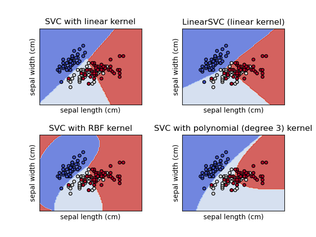
Plot different SVM classifiers in the iris dataset

https://scikit-learn.org/stable/auto_examples/svm/plot_iris_svc.html#sphx-glr-auto-examples-svm-plot-iris-svc-py

测试不同SVM分类器在iris数据上的效果。

Comparison of different linear SVM classifiers on a 2D projection of the iris dataset. We only consider the first 2 features of this dataset:

• Sepal length

• Sepal width

This example shows how to plot the decision surface for four SVM classifiers with different kernels.

The linear models LinearSVC() and SVC(kernel='linear') yield slightly different decision boundaries. This can be a consequence of the following differences:

• LinearSVC minimizes the squared hinge loss while SVC minimizes the regular hinge loss.

• LinearSVC uses the One-vs-All (also known as One-vs-Rest) multiclass reduction while SVC uses the One-vs-One multiclass reduction.

Both linear models have linear decision boundaries (intersecting hyperplanes) while the non-linear kernel models (polynomial or Gaussian RBF) have more flexible non-linear decision boundaries with shapes that depend on the kind of kernel and its parameters.

 

 

print(__doc__)

import numpy as np
import matplotlib.pyplot as plt
from sklearn import svm, datasets


def make_meshgrid(x, y, h=.02):
    """Create a mesh of points to plot in

    Parameters
    ----------
    x: data to base x-axis meshgrid on
    y: data to base y-axis meshgrid on
    h: stepsize for meshgrid, optional

    Returns
    -------
    xx, yy : ndarray
    """
    x_min, x_max = x.min() - 1, x.max() + 1
    y_min, y_max = y.min() - 1, y.max() + 1
    xx, yy = np.meshgrid(np.arange(x_min, x_max, h),
                         np.arange(y_min, y_max, h))
    return xx, yy


def plot_contours(ax, clf, xx, yy, **params):
    """Plot the decision boundaries for a classifier.

    Parameters
    ----------
    ax: matplotlib axes object
    clf: a classifier
    xx: meshgrid ndarray
    yy: meshgrid ndarray
    params: dictionary of params to pass to contourf, optional
    """
    Z = clf.predict(np.c_[xx.ravel(), yy.ravel()])
    Z = Z.reshape(xx.shape)
    out = ax.contourf(xx, yy, Z, **params)
    return out


# import some data to play with
iris = datasets.load_iris()
# Take the first two features. We could avoid this by using a two-dim dataset
X = iris.data[:, :2]
y = iris.target

# we create an instance of SVM and fit out data. We do not scale our
# data since we want to plot the support vectors
C = 1.0  # SVM regularization parameter
models = (svm.SVC(kernel='linear', C=C),
          svm.LinearSVC(C=C, max_iter=10000),
          svm.SVC(kernel='rbf', gamma=0.7, C=C),
          svm.SVC(kernel='poly', degree=3, gamma='auto', C=C))
models = (clf.fit(X, y) for clf in models)

# title for the plots
titles = ('SVC with linear kernel',
          'LinearSVC (linear kernel)',
          'SVC with RBF kernel',
          'SVC with polynomial (degree 3) kernel')

# Set-up 2x2 grid for plotting.
fig, sub = plt.subplots(2, 2)
plt.subplots_adjust(wspace=0.4, hspace=0.4)

X0, X1 = X[:, 0], X[:, 1]
xx, yy = make_meshgrid(X0, X1)

for clf, title, ax in zip(models, titles, sub.flatten()):
    plot_contours(ax, clf, xx, yy,
                  cmap=plt.cm.coolwarm, alpha=0.8)
    ax.scatter(X0, X1, c=y, cmap=plt.cm.coolwarm, s=20, edgecolors='k')
    ax.set_xlim(xx.min(), xx.max())
    ax.set_ylim(yy.min(), yy.max())
    ax.set_xlabel('Sepal length')
    ax.set_ylabel('Sepal width')
    ax.set_xticks(())
    ax.set_yticks(())
    ax.set_title(title)

plt.show()

 

Regression

支持向量方法也可以用于回归， 叫支持向量回归。

支持向量分类依赖支持向量， 此向量是在margin中， 损失函数只用这些样本来计算。

类似地， SVR也依赖训练样本的一个子集， 损失函数的计算忽略 那些预测和目标 接近的样本。

 

The method of Support Vector Classification can be extended to solve regression problems. This method is called Support Vector Regression.

The model produced by support vector classification (as described above) depends only on a subset of the training data, because the cost function for building the model does not care about training points that lie beyond the margin.

 

Analogously, the model produced by Support Vector Regression depends only on a subset of the training data, because the cost function ignores samples whose prediction is close to their target.

 

There are three different implementations of Support Vector Regression: SVR, NuSVR and LinearSVR. LinearSVR provides a faster implementation than SVR but only considers the linear kernel, while NuSVR implements a slightly different formulation than SVR and LinearSVR. See Implementation details for further details.

As with classification classes, the fit method will take as argument vectors X, y, only that in this case y is expected to have floating point values instead of integer values:

 

>>> from sklearn import svm
>>> X = [[0, 0], [2, 2]]
>>> y = [0.5, 2.5]
>>> regr = svm.SVR()
>>> regr.fit(X, y)
SVR()
>>> regr.predict([[1, 1]])
array([1.5])

 

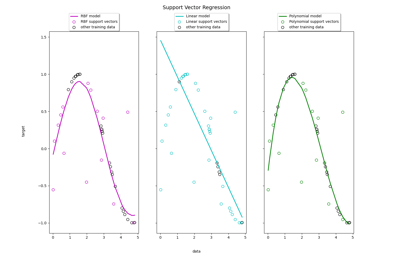
Support Vector Regression (SVR) using linear and non-linear kernels

https://scikit-learn.org/stable/auto_examples/svm/plot_svm_regression.html#sphx-glr-auto-examples-svm-plot-svm-regression-py

生成sin数据，

演示 RBF 模型 ， 线性模型 和 多项式模型的 拟合能力。

Toy example of 1D regression using linear, polynomial and RBF kernels.

 

print(__doc__)

import numpy as np
from sklearn.svm import SVR
import matplotlib.pyplot as plt

# #############################################################################
# Generate sample data
X = np.sort(5 * np.random.rand(40, 1), axis=0)
y = np.sin(X).ravel()

# #############################################################################
# Add noise to targets
y[::5] += 3 * (0.5 - np.random.rand(8))

# #############################################################################
# Fit regression model
svr_rbf = SVR(kernel='rbf', C=100, gamma=0.1, epsilon=.1)
svr_lin = SVR(kernel='linear', C=100, gamma='auto')
svr_poly = SVR(kernel='poly', C=100, gamma='auto', degree=3, epsilon=.1,
               coef0=1)

# #############################################################################
# Look at the results
lw = 2

svrs = [svr_rbf, svr_lin, svr_poly]
kernel_label = ['RBF', 'Linear', 'Polynomial']
model_color = ['m', 'c', 'g']

fig, axes = plt.subplots(nrows=1, ncols=3, figsize=(15, 10), sharey=True)
for ix, svr in enumerate(svrs):
    axes[ix].plot(X, svr.fit(X, y).predict(X), color=model_color[ix], lw=lw,
                  label='{} model'.format(kernel_label[ix]))
    axes[ix].scatter(X[svr.support_], y[svr.support_], facecolor="none",
                     edgecolor=model_color[ix], s=50,
                     label='{} support vectors'.format(kernel_label[ix]))
    axes[ix].scatter(X[np.setdiff1d(np.arange(len(X)), svr.support_)],
                     y[np.setdiff1d(np.arange(len(X)), svr.support_)],
                     facecolor="none", edgecolor="k", s=50,
                     label='other training data')
    axes[ix].legend(loc='upper center', bbox_to_anchor=(0.5, 1.1),
                    ncol=1, fancybox=True, shadow=True)

fig.text(0.5, 0.04, 'data', ha='center', va='center')
fig.text(0.06, 0.5, 'target', ha='center', va='center', rotation='vertical')
fig.suptitle("Support Vector Regression", fontsize=14)
plt.show()

 

numpy.setdiff1d

https://numpy.org/doc/stable/reference/generated/numpy.setdiff1d.html

Find the set difference of two arrays.

Return the unique values in ar1 that are not in ar2.

a = np.array([1, 2, 3, 2, 4, 1])

b = np.array([3, 4, 5, 6])

np.setdiff1d(a, b)
array([1, 2])

 

Tips on Practical Use

如果有大量的噪音，应该降低 C 值， 加重正则化效果。

• Setting C: C is 1 by default and it’s a reasonable default choice. If you have a lot of noisy observations you should decrease it: decreasing C corresponds to more regularization.

  LinearSVC and LinearSVR are less sensitive to C when it becomes large, and prediction results stop improving after a certain threshold. Meanwhile, larger C values will take more time to train, sometimes up to 10 times longer, as shown in 11.

SVM对数据的伸缩性不变的， 必须先进行伸缩。

• Support Vector Machine algorithms are not scale invariant, so it is highly recommended to scale your data. For example, scale each attribute on the input vector X to [0,1] or [-1,+1], or standardize it to have mean 0 and variance 1. Note that the same scaling must be applied to the test vector to obtain meaningful results. This can be done easily by using a Pipeline:

  >>>

  >>> from sklearn.pipeline import make_pipeline
  >>> from sklearn.preprocessing import StandardScaler
  >>> from sklearn.svm import SVC
  
  >>> clf = make_pipeline(StandardScaler(), SVC())
  

  See section Preprocessing data for more details on scaling and normalization.

如果数据不均衡，需要设置对应参数。

In SVC, if the data is unbalanced (e.g. many positive and few negative), set class_weight='balanced' and/or try different penalty parameters C.