Neural Style论文笔记+源码解析
引言
前面在Ubuntu16.04+GTX1080配置TensorFlow并实现图像风格转换中介绍了TensorFlow的配置过程,以及运用TensorFlow实现图像风格转换,主要是使用了文章A Neural Algorithm of Artistic Style中的方法,今天,我将主要对这篇文章进行解读,并对基于TensorFlow版本的Neural Style开源代码进行解析。
论文地址:A Neural Algorithm of Artistic Style
源码地址:Neural Style in TensorFlow
A Neural Algorithm of Artistic Style
任意一幅画,在人的眼中可以分为两个部分,一是画的具体内容(Content),如人物、山水、建筑等等,这是很实在的东西;二是绘画的风格(Style),这却是很抽象的东西,这和艺术家的手法、使用的绘画材料以及绘画习惯都有很大的关系。而在计算机中,这仅仅是一些像素点(pixel)而已。这篇文章的key finding是the representations of content and style in the Convolutional Neural Network are separable,即,我们不仅仅可以用深度学习来提取图像的特征,同时还可以将图像的Content和Style分隔开来。
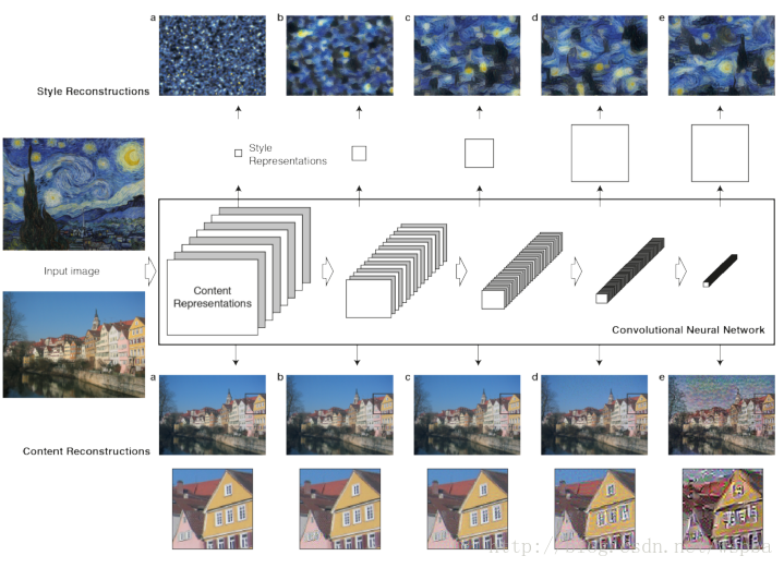
上图即代表了这篇文章的整体框架。
这里的CNN模型使用的是pre-trained的VGG-16模型。
主要包含两个部分:
Content Reconstruction:将图像输入到CNN模型中,使用不同的layer提取到的feature maps来对输入图像进行reconstruct。上图中使用了VGG的‘conv1_1’(a), ‘conv2_1’(b), ‘conv3_1’(c), ‘conv4_1’(d) 和‘conv5_1’(e)的feature maps来重构原始图像。作者在文中说,使用低层的特征能够很好的对原始图像的像素值进行重构(a,b,c),而使用高层的特征来重构的时候detailed pixel出现了丢失,但是图像中的high-level content却保留了下来(d,e),因此认为高层的特征能够更好的对图像的content进行重构。
Style Reconstruction:Style 的重构比Content复杂的多,作者提出使用某一层不同filter的响应之间的correlations来代表该层提取到的texture information,然后来对Style进行重构。上图中使用了VGG的
‘conv1_1’(a), ‘conv1_1’+‘conv2_1’(b), ‘conv1_1’+‘conv2_1’ +‘conv3_1’(c),‘conv1_1’+‘conv2_1’+‘conv3_1’+‘conv4_1’(d), ‘conv1_1’+‘conv2_1’+‘conv3_1’+‘conv4_1’+‘conv5_1’(e)的texture information来进行重构。作者表示使用多层的feature correlations来重构的Style会在各个不同的尺度上更加匹配图像本身的style,忽略场景的全局信息。
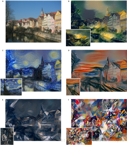
基于以上,作者提出了本文的主要工作:finding an image that simultaneously matches the content representation of the photograph and the style representation of the artwork,即将一幅画的Style和另一幅话的Content进行融合,来证明作者的观点。
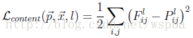
假设某一层得到的响应是Fl∈RNl∗MlFl∈RNl∗Ml,其中NlNl为l层filter的个数,MlMl为filter的大小。FlijFijl表示的是第l层第i个filter在位置j的输出。
p⃗ p→代表提供Content的图像,x⃗ x→表示生成的图像,PlPl和FlFl分别代表它们对于l层的响应,因此l层的Content Loss:
上面我们提到了,某一层的Style可以用Gl∈RNl∗NlGl∈RNl∗Nl来表示,其中Glij=∑kFlik∗FljkGijl=∑kFikl∗Fjkl,即不同filter响应的内积。
a⃗ a→代表提供Style的图像,x⃗ x→表示生成的图像,AlAl和GlGl分别代表它们对于l层的Style,因此l层的Style Loss: 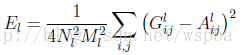
文章中作者使用了多层来表达Style,所以总的Style Loss为: 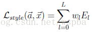
定义好了两个Loss之后,就利用优化方法来最小化总的Loss: 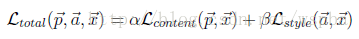
其中的αα和ββ分别代表了对Content和Style的侧重,文中作者也对α/βα/β取值的效果进行了实验。
最终迭代出来的x⃗ x→既具有p⃗ p→的Content,同时也具有a⃗ a→的Style。实验结果也证明了作者文中方法的有效性。
Neural Style in TensorFlow
TensorFlow版本的源码主要包含了三个文件:neural_style.py, stylize.py和 vgg.py。
neural_style.py:外部接口函数,定义了函数的主要参数以及部分参数的默认值,包含对图像的读取和存贮,对输入图像进行resize,权值分配等操作,并将参数以及resize的图片传入stylize.py中。
stylize.py:核心代码,包含了训练、优化等过程。
vgg.py:定义了网络模型以及相关的运算。
以下主要对stylize.py中的相关代码进行解析。
shape = (1,) + content.shape
style_shapes = [(1,) + style.shape for style in styles]- 1
- 2
content.shape是三维(height, width, channel),这里将维度变成(1, height, width, channel)为了与后面保持一致。
# compute content features in feedforward mode
g = tf.Graph() #创建图
    with g.as_default(), g.device('/cpu:0'), tf.Session() as sess:
        image = tf.placeholder('float', shape=shape)
        net, mean_pixel = vgg.net(network, image)
        content_pre = np.array([vgg.preprocess(content, mean_pixel)])
content_features[CONTENT_LAYER] = net[CONTENT_LAYER].eval(feed_dict={image: content_pre})- 1
- 2
- 3
- 4
- 5
- 6
- 7
首先创建一个image的占位符,然后通过eval()的feed_dict将content_pre传给image,启动net的运算过程,得到了content的feature maps。
# compute style features in feedforward mode
    for i in range(len(styles)):
        g = tf.Graph()
        with g.as_default(), g.device('/cpu:0'), tf.Session() as sess:
            image = tf.placeholder('float', shape=style_shapes[i])
            net, _ = vgg.net(network, image)
            style_pre = np.array([vgg.preprocess(styles[i], mean_pixel)])
            for layer in STYLE_LAYERS:
                features = net[layer].eval(feed_dict={image: style_pre})
                features = np.reshape(features, (-1, features.shape[3]))
                gram = np.matmul(features.T, features) / features.size
style_features[i][layer] = gram- 1
- 2
- 3
- 4
- 5
- 6
- 7
- 8
- 9
- 10
- 11
- 12
由于style图像可以输入多幅,这里使用for循环。同样的,将style_pre传给image占位符,启动net运算,得到了style的feature maps,由于style为不同filter响应的内积,因此在这里增加了一步:gram = np.matmul(features.T, features) / features.size,即为style的feature。
# make stylized image using backpropogation
    with tf.Graph().as_default():
        if initial is None:
            noise = np.random.normal(size=shape, scale=np.std(content) * 0.1)
            initial = tf.random_normal(shape) * 0.256
        else:
            initial = np.array([vgg.preprocess(initial, mean_pixel)])
            initial = initial.astype('float32')
        image = tf.Variable(initial)
        net, _ = vgg.net(network, image)

        # content loss
        content_loss = content_weight * (2 * tf.nn.l2_loss(
                net[CONTENT_LAYER] - content_features[CONTENT_LAYER]) / content_features[CONTENT_LAYER].size)
        # style loss
        style_loss = 0
        for i in range(len(styles)):
            style_losses = []
            for style_layer in STYLE_LAYERS:
                layer = net[style_layer]
                _, height, width, number = map(lambda i: i.value, layer.get_shape())
                size = height * width * number
                feats = tf.reshape(layer, (-1, number))
                gram = tf.matmul(tf.transpose(feats), feats) / size
                style_gram = style_features[i][style_layer]
                style_losses.append(2 * tf.nn.l2_loss(gram - style_gram) / style_gram.size)
            style_loss += style_weight * style_blend_weights[i] * reduce(tf.add, style_losses)
        # total variation denoising
        tv_y_size = _tensor_size(image[:,1:,:,:])
        tv_x_size = _tensor_size(image[:,:,1:,:])
        tv_loss = tv_weight * 2 * (
                (tf.nn.l2_loss(image[:,1:,:,:] - image[:,:shape[1]-1,:,:]) /
                    tv_y_size) +
                (tf.nn.l2_loss(image[:,:,1:,:] - image[:,:,:shape[2]-1,:]) /
                    tv_x_size))
        # overall loss
loss = content_loss + style_loss + tv_loss- 1
- 2
- 3
- 4
- 5
- 6
- 7
- 8
- 9
- 10
- 11
- 12
- 13
- 14
- 15
- 16
- 17
- 18
- 19
- 20
- 21
- 22
- 23
- 24
- 25
- 26
- 27
- 28
- 29
- 30
- 31
- 32
- 33
- 34
- 35
- 36
- 37
image = tf.Variable(initial)初始化了一个TensorFlow的变量,即为我们需要训练的对象。注意这里我们训练的对象是一张图像,而不是weight和bias。接下来定义了Content Loss和Style Loss,结合文中的公式很容易看懂,在代码中,还增加了total variation denoising,因此总的loss = content_loss + style_loss + tv_loss。
# optimizer setup
train_step = tf.train.AdamOptimizer(learning_rate).minimize(loss)- 1
- 2
创建train_step,使用Adam优化器,优化对象是上面的loss。
# optimization
        best_loss = float('inf')
        best = None
        with tf.Session() as sess:
            sess.run(tf.initialize_all_variables())
            for i in range(iterations):
                last_step = (i == iterations - 1)
                print_progress(i, last=last_step)
                train_step.run()

                if (checkpoint_iterations and i % checkpoint_iterations == 0) or last_step:
                    this_loss = loss.eval()
                    if this_loss < best_loss:
                        best_loss = this_loss
                        best = image.eval()
                    yield (
                        (None if last_step else i),
                        vgg.unprocess(best.reshape(shape[1:]), mean_pixel)
)- 1
- 2
- 3
- 4
- 5
- 6
- 7
- 8
- 9
- 10
- 11
- 12
- 13
- 14
- 15
- 16
- 17
- 18
- 19
优化过程,通过迭代使用train_step来最小化loss,最终得到一个best,即为训练优化的结果。
总的来说,TensorFlow是一个效率很高、功能很强大的工具,代码也并不是很难看懂,本人对TensorFlow并不是很熟悉,还需要对它的内部函数以及运行机制更深入的了解,因此这也当做是一个学习的过程,上述如果有任何不对的地方,也希望大家批评指正。

 浙公网安备 33010602011771号