学习笔记(六): Regularization for Simplicity
目录
Overcrossing?
complete this exercise that explores overuse of feature crosses.
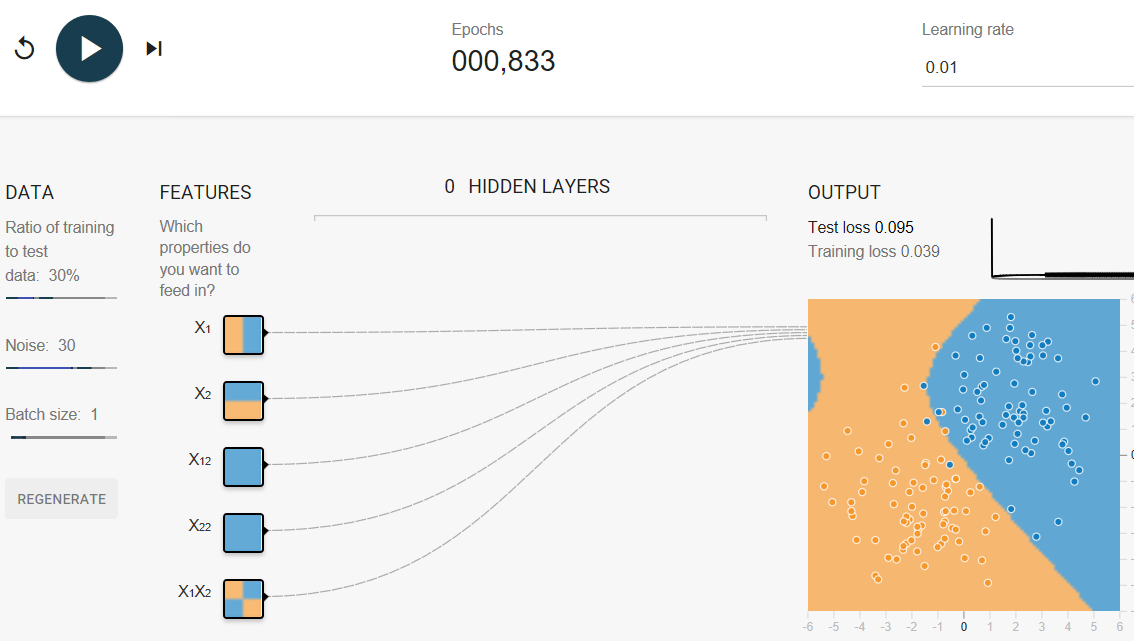
Task 1: Run the model as is, with all of the given cross-product features. Are there any surprises in the way the model fits the data? What is the issue?
overcrossing
▾answer to Task 1.
Surprisingly, the model's decision boundary looks kind of crazy. In particular, there's a region in the upper left that's hinting towards blue, even though there's no visible support for that in the data.
Notice the relative thickness of the five lines running from INPUT to OUTPUT. These lines show the relative weights of the five features. The lines emanating发射 from X1 and X2 are much thicker密集(权重更大) than those coming from the feature crosses. So, the feature crosses are contributing far less to the model than the normal (uncrossed) features.
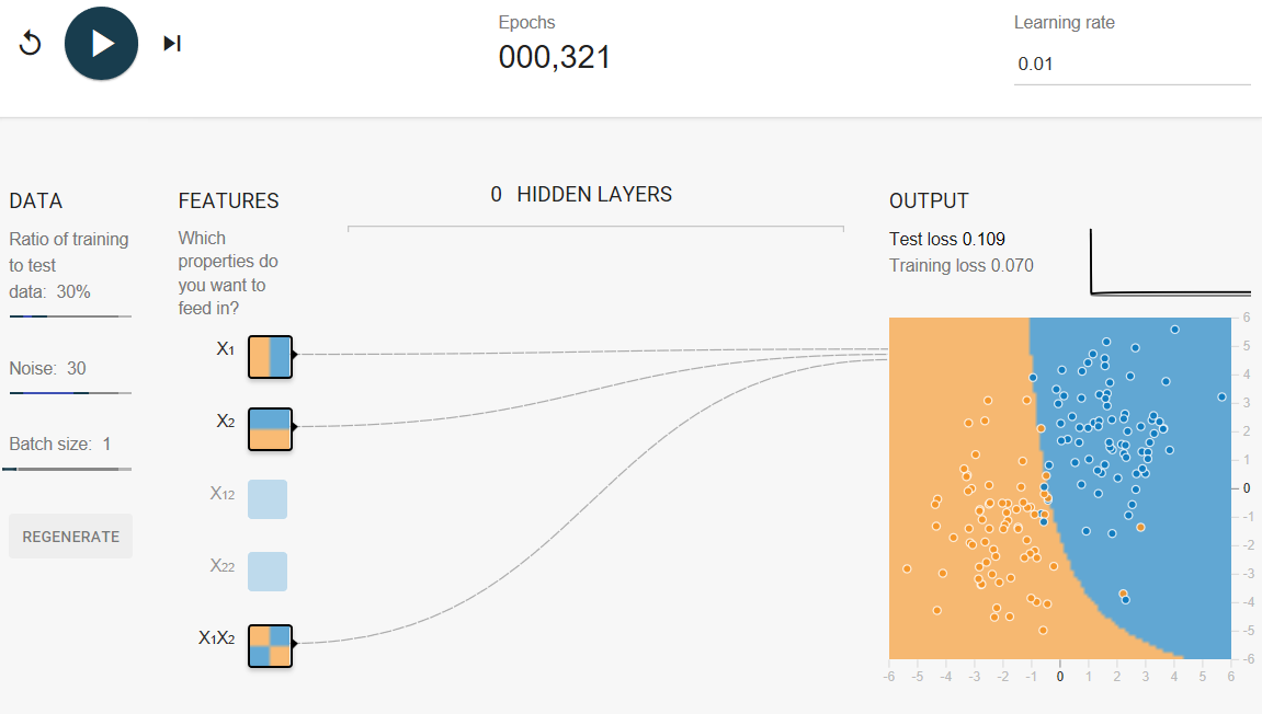
Task 2: Try removing various cross-product features to improve performance (albeit尽管 only slightly). Why would removing features improve performance?
Removing feature crosses
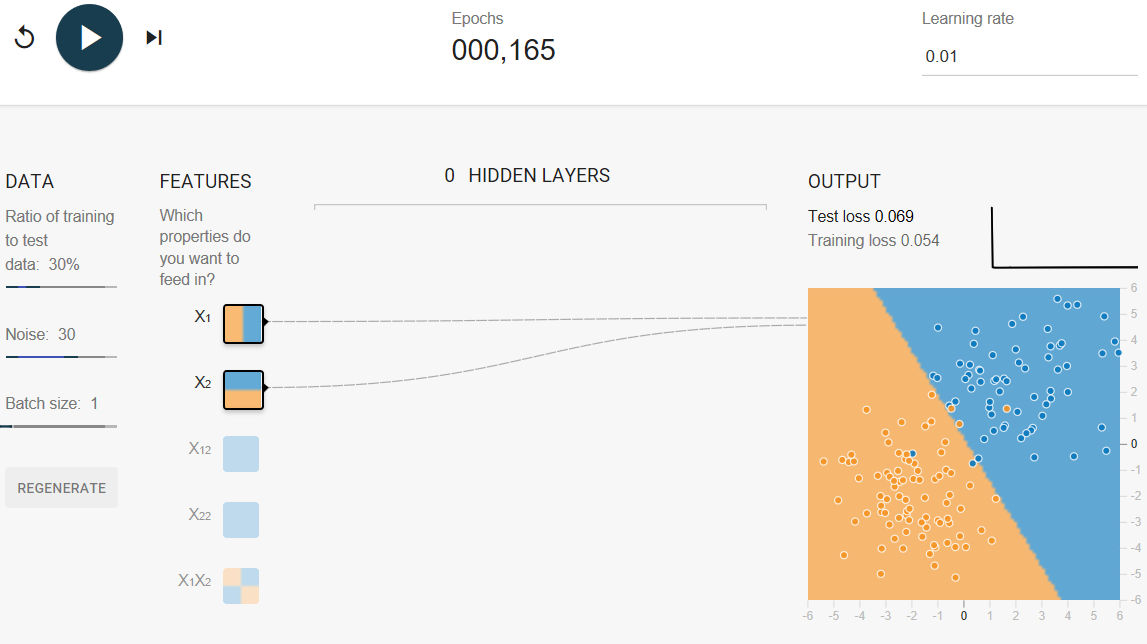
Removing all the feature crosses
▾answer to Task 2.
Removing all the feature crosses gives a saner合理 model (there is no longer a curved boundary suggestive of overfitting) and makes the test loss converge.
After 1,000 iterations, test loss should be a slightly lower value than when the feature crosses were in play (although your results may vary a bit, depending on the data set).
The data in this exercise is basically linear data plus noise. If we use a model that is too complicated, such as one with too many crosses, we give it the opportunity to fit to the noise in the training data, often at the cost of making the model perform badly on test data.
L₂ Regularization
Consider the following generalization curve, which shows the loss for both the training set and validation set against the number of training iterations.
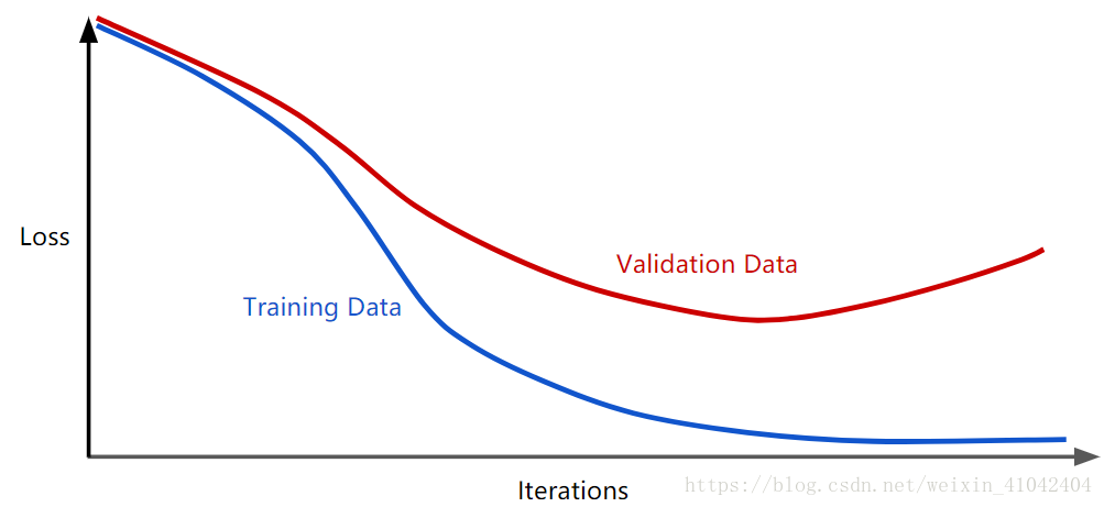
Figure 1. Loss on training set and validation set.
Figure 1 shows a model in which training loss gradually decreases, but validation loss eventually goes up. In other words, this generalization curve shows that the model is overfitting to the data in the training set. Channeling our inner Ockham奥卡姆, perhaps we could prevent overfitting by penalizing complex models, a principle called regularization.
In other words, instead of simply aiming to minimize loss (empirical risk minimization):
we'll now minimize loss+complexity, which is called structural risk minimization:
Our training optimization algorithm is now a function of two terms: the loss term, which measures how well the model fits the data, and the regularization term, which measures model complexity.
Machine Learning Crash Course focuses on two common (and somewhat related) ways to think of model complexity:
- Model complexity as a function of the weights of all the features in the model.
- Model complexity as a function of the total number of features with nonzero weights. (A later module covers this approach.)
If model complexity is a function of weights, a feature weight with a high absolute value is more complex than a feature weight with a low absolute value.
We can quantify complexity using the L2 regularization formula, which defines the regularization term as the sum of the squares of all the feature weights:
In this formula, weights close to zero have little effect on model complexity, while outlier weights can have a huge impact.
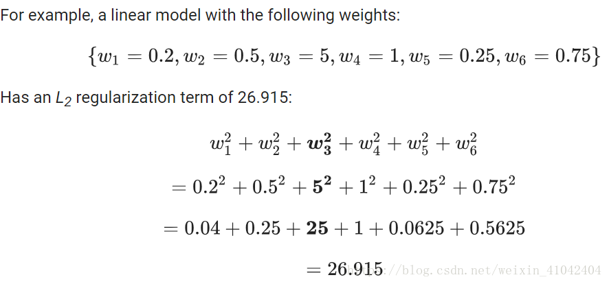
But w3 (bolded above), with a squared value of 25, contributes nearly all the complexity. The sum of the squares of all five other weights adds just 1.915 to the L2 regularization term.
Lambda
Model developers tune the overall impact of the regularization term by multiplying its value by a scalar标量 known as lambda (also called the regularization rate). That is, model developers aim to do the following:

Performing L2 regularization has the following effect on a model
- Encourages weight values toward 0 (but not exactly 0)
- Encourages the mean of the weights toward 0, with a normal (bell-shaped or Gaussian) distribution.
Increasing the lambda value strengthens the regularization effect. For example, the histogram of weights for a high value of lambda might look as shown in Figure 2.
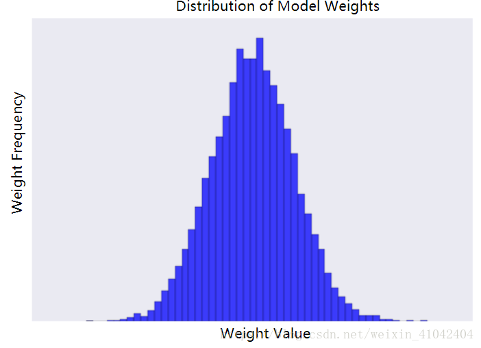
Figure 2. Histogram of weights.
Lowering the value of lambda tends to yield a flatter histogram, as shown in Figure 3.

Figure 3. Histogram of weights produced by a lower lambda value.
When choosing a lambda value, the goal is to strike the right balance between simplicity and training-data fit:
-
If your lambda value is too high, your model will be simple, but you run the risk of underfitting your data. Your model won't learn enough about the training data to make useful predictions.
-
If your lambda value is too low, your model will be more complex, and you run the risk of overfitting your data. Your model will learn too much about the particularities of the training data, and won't be able to generalize to new data.
Note: Setting lambda to zero removes regularization completely. In this case, training focuses exclusively on minimizing loss, which poses the highest possible overfitting risk.
The ideal value of lambda produces a model that generalizes well to new, previously unseen data. Unfortunately, that ideal value of lambda is data-dependent, so you'll need to do some tuning.
▾learn about L2 regularization and learning rate.
There's a close connection between learning rate and lambda. Strong L2 regularization values tend to drive feature weights closer to 0. Lower learning rates (with early stopping) often produce the same effect because the steps away from 0 aren't as large. Consequently, tweaking learning rate and lambda simultaneously may have confounding effects.
Early stopping means ending training before the model fully reaches convergence. In practice, we often end up with some amount of implicit early stopping when training in an online(continuous) fashion. That is, some new trends just haven't had enough data yet to converge.
As noted, the effects from changes to regularization parameters can be confounded with the effects from changes in learning rate or number of iterations. One useful practice (when training across a fixed batch of data) is to give yourself a high enough number of iterations that early stopping doesn't play into things.
Examining L2 regularization
Increasing the regularization rate from 0 to 0.3 produces the following effects:
1.Test loss drops significantly.
Note: While test loss decreases, training loss actually increases. This is expected, because you've added another term to the loss function to penalize complexity. Ultimately, all that matters is test loss, as that's the true measure of the model's ability to make good predictions on new data.
2.The delta between Test loss and Training loss drops significantly.
3.The weights of the features and some of the feature crosses have lower absolute values, which implies that model complexity drops.
Check Understanding
1.L2 Regularization
Imagine a linear model with 100 input features:
Which of the following statements are true?
-
-
10 are highly informative.
-
90 are non-informative.
-
Assume that all features have values between -1 and 1.
-
(T)L2 regularization will encourage many of the non-informative weights to be nearly (but not exactly) 0.0.
(T)L2 regularization may cause the model to learn a moderate weight for some non-informative features.(Surprisingly, this can happen when a non-informative feature happens to be correlated with the label. In this case, the model incorrectly gives such non-informative features some of the "credit" that should have gone to informative features.)
(F)L2 regularization will encourage most of the non-informative weights to be exactly 0.0.(L2 regularization penalizes larger weights more than smaller weights. As a weight gets close to 0.0, L2 "pushes" less forcefully toward 0.0. )
2.L2 Regularization and Correlated Features
Imagine a linear model with two strongly correlated features; these two features are nearly identical copies of one another but one feature contains a small amount of random noise. If we train this model with L2 regularization, what will happen to the weights for these two features?
(F)One feature will have a large weight; the other will have a weight of almost 0.0.
(T)Both features will have roughly equal, moderate weights.(L2 regularization will force the features towards roughly equivalent weights that are approximately half of what they would have been had only one of the two features been in the model.)
(F)One feature will have a large weight; the other will have a weight of exactly 0.0.
Glossay
1.structural risk minimization (SRM):
An algorithm that balances two goals:
- The desire to build the most predictive model (for example, lowest loss).
- The desire to keep the model as simple as possible (for example, strong regularization).
For example, a function that minimizes loss+regularization on the training set is a structural risk minimization algorithm.
For more information, see http://www.svms.org/srm/.
Contrast with empirical risk minimization.
2.regularization:
The penalty on a model's complexity. Regularization helps prevent overfitting. Different kinds of regularization include:
- L1 regularization
- L2 regularization
- dropout regularization
- early stopping (this is not a formal regularization method, but can effectively limit overfitting)
3.L1 regularization:
A type of regularization that penalizes weights in proportion to the sum of the absolute values of the weights. In models relying on sparse features, L1 regularization helps drive the weights of irrelevant or barely relevant features to exactly 0, which removes those features from the model. Contrast with L2 regularization.
4.L2 regularization:
A type of regularization that penalizes weights in proportion to the sum of the squares of the weights. L2 regularization helps drive outlier weights (those with high positive or low negative values) closer to 0 but not quite to 0. (Contrast with L1 regularization.) L2 regularization always improves generalization in linear models.
5.lambda:
Synonym for regularization rate.
(This is an overloaded term. Here we're focusing on the term's definition within regularization.)
6.regularization rate:
A scalar value, represented as lambda, specifying the relative importance of the regularization function. The following simplified loss equation shows the regularization rate's influence:
minimize(loss function + λ(regularization function))
Raising the regularization rate reduces overfitting but may make the model less accurate.
7.early stopping:
A method for regularization that involves ending model training before training loss finishes decreasing. In early stopping, you end model training when the loss on a validation data set starts to increase, that is, when generalization performance worsens.

 浙公网安备 33010602011771号