Motion Planning for Mobile Robots 学习笔记2
What this note covers
- 第1节:图搜索基础
任务1:图搜索基础(Graph Search Basis) - 第2节:Dijkstra和A*算法
任务2:Djkstra和A*算法(Djkstra and A*) - 第3节:JPS算法
任务3:JPS算法(Jump Point Search) - 第4节:作业
任务4:实践演示
Graph Search Basis
Configuration Space
配置空间
- Robot configuration
机器人配置:a specifcation of the positions of all points of the robot
对机器人上所有点位置的描述 - Robot degree of freedom(DOF)
The minimum number n of real-valued coordinates needed to represent the robot configuration
自由度:用最少的坐标数量表示机器人可能存在的配置 - Robot configuration space
a n-dim space containing all possible robot configurations,
denoted as C-space
机器人的配置空间:N(自由度)维空间,其中包含了机器人所有可能存在的配置 - Each robot pose is a point in the C-space
机器人任一位置对应配置空间中的一个点
Configuration Space Obstacle
配置空间中的障碍物
Planning in workspace
工作空间(机器人所处的复杂环境)中的规划
-
Robot has different shape and size
机器人有不同的形状与大小 -
Collision detection requires knowing the robot geometry - time consuming and hard
需要知道机器人的几何形状以进行碰撞检测,耗费时间且实现复杂
Planning in configuration space
-
Robot is represented by a point in C-space, e.g. position (a point in \(R^3\)), pose (a point in So(3)), etc.
机器人任一位置对应配置空间中的一个点
position指机器人位置,是\(R^3\)空间中的一个点。
pose指机器人六自由度的姿态,是SO(3)空间中的一个点。 -
Obstacles need to be represented in configuration space (one-time work prior to motion planning), called configuration space obstacle, or C-obstacle
C-obstacle指配置空间中的障碍物,这是规划前的一次性工作
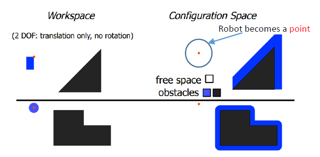
地面的小车可认为是方形
空中无人机与扫地机器人可认为是圆形
-
C-space = (C-obstacle) \(\cup\) (C-free)
-
The path planning is finding a path between start point \(q_start\) and goal point \(q_goal\) within C-free
Graph and Search Method
Graphs
什么是图?
图是节点与边组成的表达方式。
边可以是有向的或无向的。
边是可以有权重的。
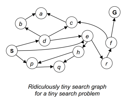
State space graph
State space graph: a mathematical representation of a search algorithm
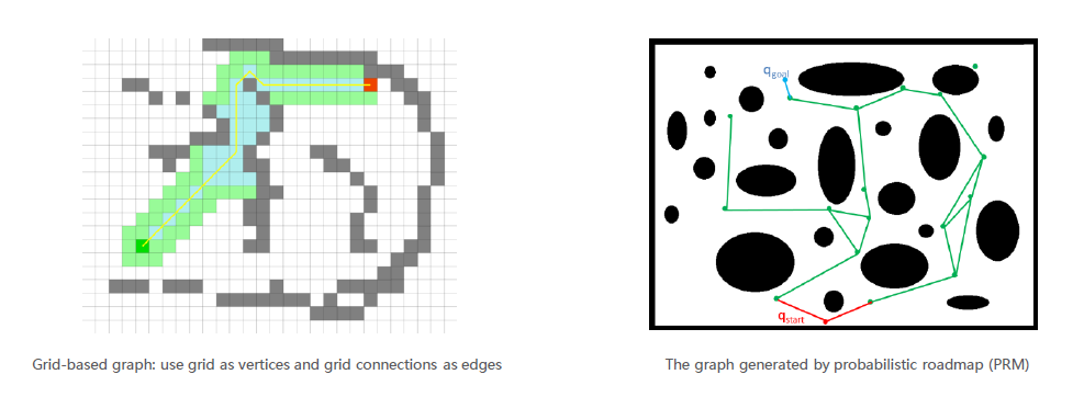
下面两个例子:
左侧是栅格地图上的路径规划问题。栅格地图上的任何节点本身与相邻节点具有连接关系,因此已经是一个图。
右侧是基于采样的路径规划方法,其图中只有黑色的障碍物,并没有类似于栅格地图一样的天然连接关系。需要构造图,例如PRM方法。
- For every search problem, there's a corresponding state space graph
- Connectivity between nodes in the graph is represented by (directed or undirected) edges
Graph Search Overview
The search always start from start state \(X_s\)
-
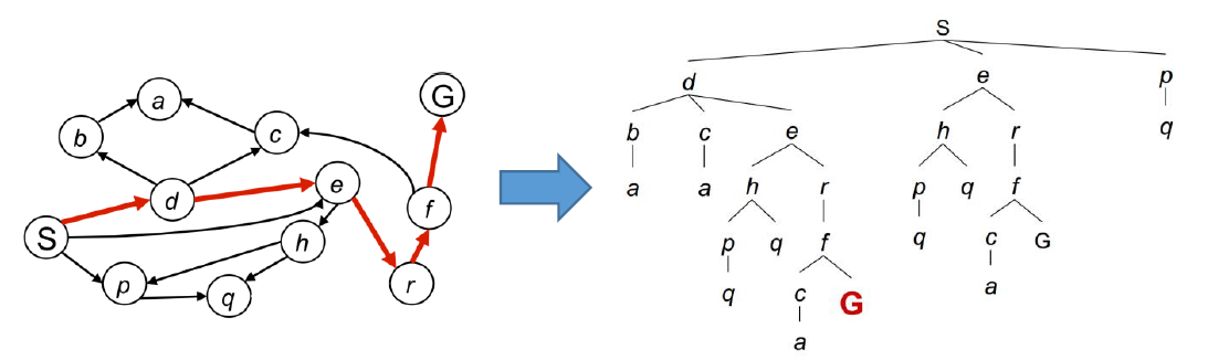
Searching the graph produces a search tree
对图进行图搜索,总是可以产生一个搜索树。
-
Back-tracing a node in the search tree gives us a path from the start state to that node
当搜索到目标后,进行回溯,即可找到一条路径。 -
For many problems we can never actually build the whole tree, too large or inefficient -we only want to reach the goal node asap.
而对于实际问题,我们很难构造整个的搜索树,只关心尽快到达目标点。
(asap, as soon as possible)
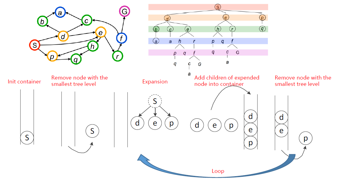
Overview
- Maintain a container to store all the nodes to be visited
维护一个容器,维护需要访问的节点 - The container is initialized with the start state \(X_s\)
在容器中加入起点以初始化 - Loop
- Remove a node from the container according to some pre-defined score function
通过预先定义的指标从容器弹出一个节点
关键问题:
按照什么规则弹出/访问节点,使得尽可能快地到达目标。
In what way to remove the right node such that the goal state can be reached as soon as possible, which results in less expansion of the graph node.
也即提高算法的效率。- Visit a node
- Expansion: Obtain all neighbors of the node
获取其所有邻居节点- Discover all its neighbors
- Push them (neighbors) into the container
将其邻居节点装入容器
- Remove a node from the container according to some pre-defined score function
- End Loop
结束条件:-
容器已空
End the loop when the container is empty -
若图存在回环,需要维护一个新的容器,其中包括所有已访问的节点(常称为close-space,闭集)。这里面的节点不会被再次访问。
When a node is removed from the container (expanded / visited), it should never be added back to the container again
-
Graph Traversal
图遍历
Basic Methods
Breadth First Search vs. Depth First Search
广度优先搜索与深度优先搜索
BFS
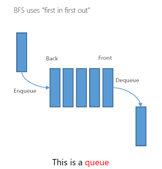
Strategy: remove / expand the shallowest node in the container
弹出容器中最浅层次的节点
container: queen
使用容器:队列
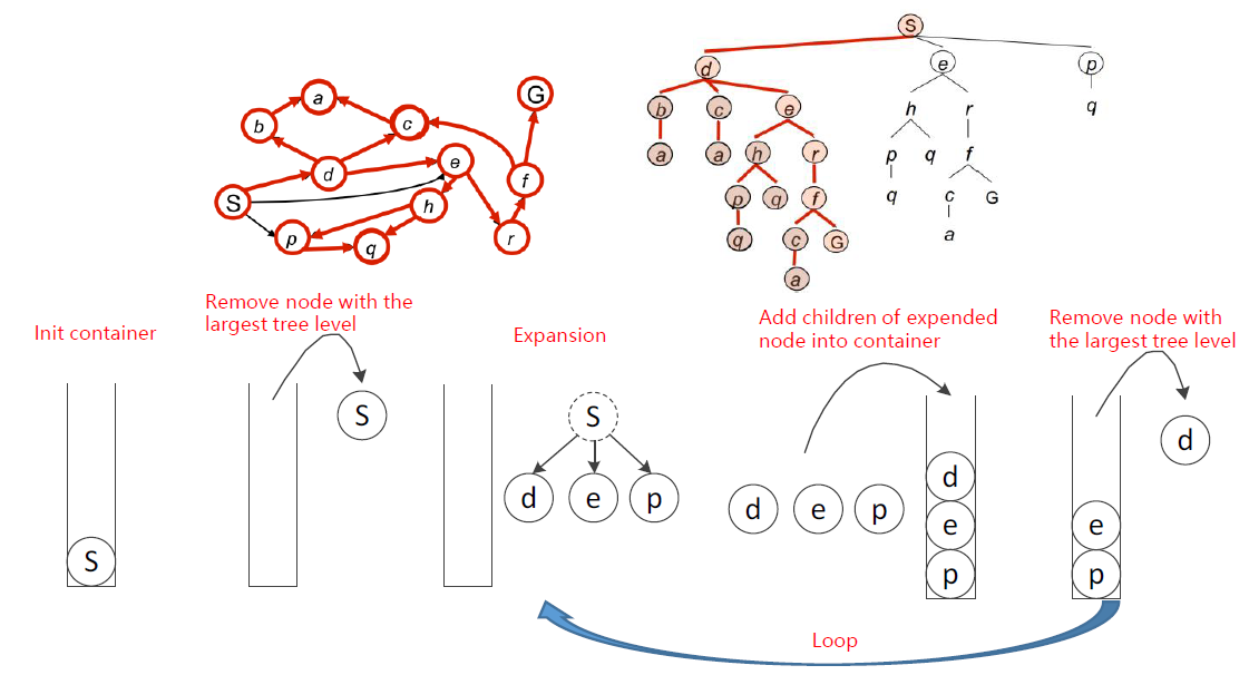
DFS
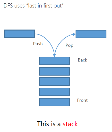
Strategy: remove / expand the deepest node in the container
弹出容器中最深层次的节点
container: stack
使用容器:栈
Heuristic Search
启发式搜索
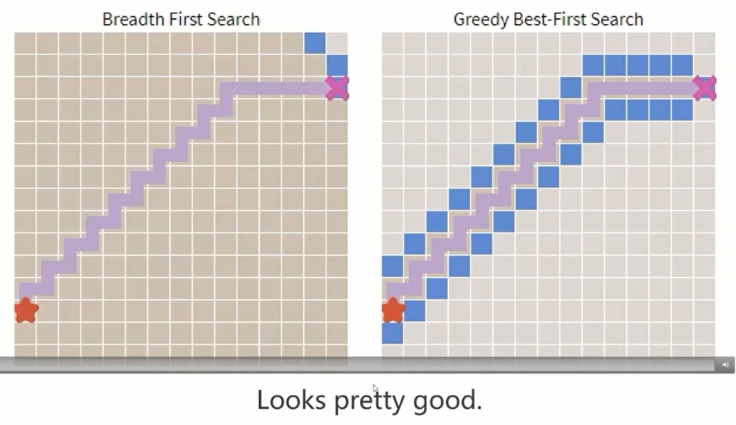
Greedy Best First Search
贪婪最佳搜索
-
BFS and DFS pick the next node off the frontiers based on which was "first in"or "last in".
主要区别还是在于选取点的规则。 -
Greedy Best First picks the "best"node according to some rule, called a heuristic.
heuristic:启发,其对每个点离终点有多近的估计。
Definition: A heuristic is a guess of how close you are to the target.
常用的猜测方法包括:Euclidean Distance(欧氏距离,即直线距离)与Manhattan Distance(曼哈顿距离,即x距离加y距离),这些都是actual shortest path的近似值。
对启发算法的要求:
- A heuristic guides you in the right direction.
指引正确的搜索方向。 - A heuristic should be easy to compute.
易于计算 。
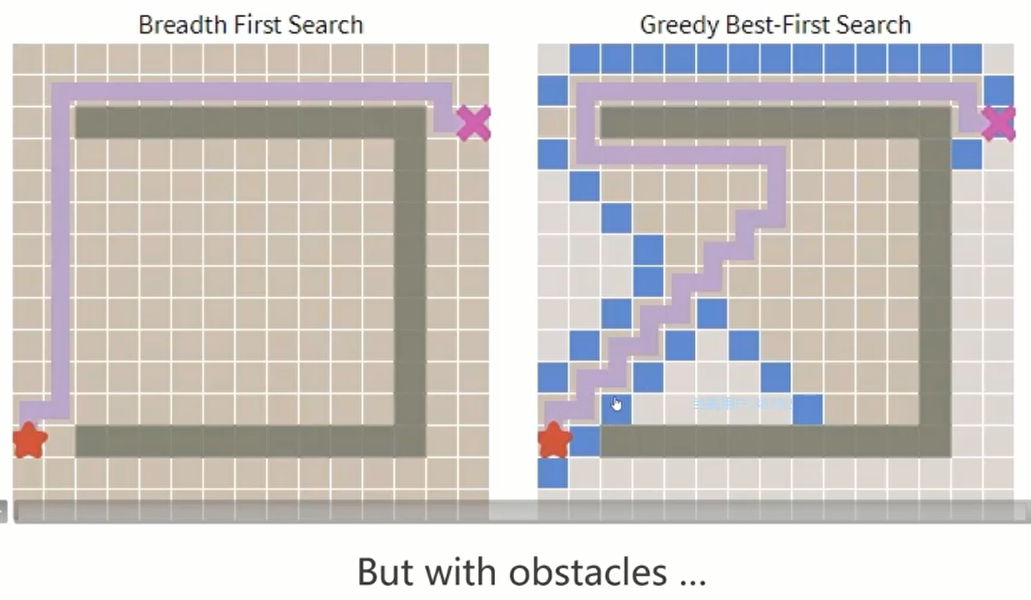
贪心算法并不是理想的算法,但是其具备很多可借鉴的性质。
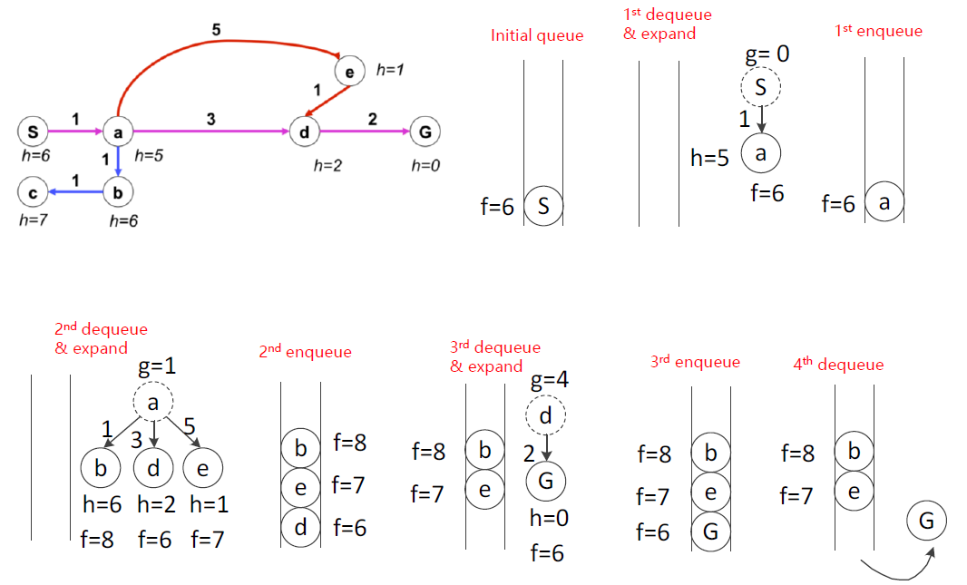
Algorithm Workflow
Cost on Actions
对于有权图,BFS无法找到路径
- A practical search problem has a cost "C" from a node to its neighbor
- Length, time, energy, etc
- When all weight are 1, BFS finds the optimal solution
- For general cases, how to find the least-cost path as soon as possible?
Dijkstra's Algorithm
Dijkstra's Algorithm Overview
- Strategy: expand/visit the node with cheapest accumulated cost g(n)
弹出节点原则:弹出具有最小函数值(累计成本,从起点到n累计的cost)g(n)的节点- g(n): The current best estimates of the accumulated cost from the start state to node "n"
- Update the accumulated costs g(m) for all unexpanded neighbors "m" of node "n"
扩展中,会检查g(m)能否用n来下降?(通过n到m,是否可使g(m)下降?) - A node that has been expanded/visited is guaranteed to have the smallest cost from the start state
Dijkstra算法最优性的保证
伪代码流程
- Maintain a priority queue to store all the nodes to be expanded
使用优先队列存储所需访问的节点
优先队列:可自动将加入的值按照从小到大顺序排列 - The priority queue is initialized with the start state \(X_s\)
初始化 - Assign g(\(X_s\))=0, and g(n)=infinite for all other nodes in the graph
初始化 - Loop
- If the queue is empty, return FALSE; break;
找不到路径 - Remove the node "n" with the lowest g(n) from the priority queue
弹出 - Mark node "n" as expanded
将其加入close-list - If the node "n" is the goal state, return TRUE; break
- For all unexpanded neighbors "m" of node "n"
- If g(m) = infinite
- g(m) = g(n) + \(C_{nm}\)
\(C_{nm}\)表示从n到m的cost - Push node "m" into the queue
- g(m) = g(n) + \(C_{nm}\)
- If g(m) > g(m) + \(C_{nm}\)
检查g(m)能否用n来下降?- g(m) =g(n) +\(C_{nm}\)
- If g(m) = infinite
- end
- If the queue is empty, return FALSE; break;
- End Loop
Pros and Cons of Dijkstra' s Algorithm
Dijkstra算法的优缺点
The good:
- Complete and optimal
完备的与最优的
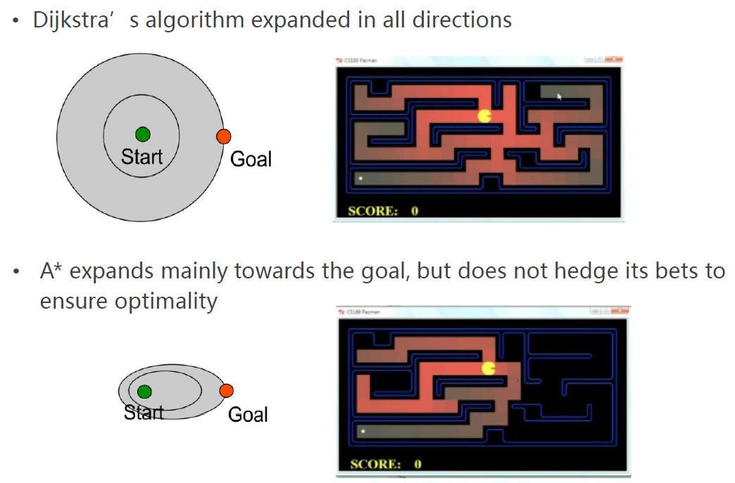
The bad: - Can only see the cost accumulated so far (i.e. the uniform cost), thus exploring next state in every "direction"
向所有方向均匀扩散 - No information about goal location
没有任何关于终点的信息
Dijkstra算法等同于带权图的BFS,当各边权重为1时,其等同于BFS。
相当于穷举
Dijkstra算法的改进
- Recall the heuristic introduced in Greedy Best First Search
- Overcome the shortcomings of uniform cost search by inferring the least cost to goal (i.e. goal cost)
- Designed for particular search problem
- Examples: Manhattan distance VS. Euclidean distance
A*: Dijkstra with a Heuristic
A* Overview
- Accumulated cost
累计代价- g(n): The current best estimates of the accumulated cost from the start state to node "n"
- Heuristic
启发函数- h(n): The estimated least cost from node n to goal state (i.e. goal cost)
- The least estimated cost from start state to goal state passing through node "n" is f(n) = g(n) +h(n)
- Strategy: expand the node with cheapest f(n) =g(n) + h(n)
弹出f值最小的n- Update the accumulated costs g(m) for all unexpanded neighbors "m" of node "n"
- A node that has been expanded is guaranteed to have the smallest cost from the start state
同样可以保证最优性
伪代码流程
- Maintain a priority queue to store all the nodes to be expanded
使用优先队列存储所需访问的节点
优先队列:可自动将加入的值按照从小到大顺序排列 - The heuristic function h(n) for all nodes are pre-defined
计算各点估计值 - The priority queue is initialized with the start state \(X_s\)
初始化 - Assign g(\(X_s\))=0, and g(n)=infinite for all other nodes in the graph
初始化 - Loop
-
If the queue is empty, return FALSE; break;
找不到路径 -
Remove the node "n" with the lowest f(n)=g(n)+h(n) from the priority queue
加粗部分是与Dijkstra算法唯一的不同之处
弹出 -
Mark node "n" as expanded
将其加入close-list -
If the node "n" is the goal state, return TRUE; break
-
For all unexpanded neighbors "m" of node "n"
- If g(m) = infinite
- g(m) = g(n) + \(C_{nm}\)
\(C_{nm}\)表示从n到m的cost - Push node "m" into the queue
- g(m) = g(n) + \(C_{nm}\)
- If g(m) > g(m) + \(C_{nm}\)
检查g(m)能否用n来下降?- g(m) =g(n) +\(C_{nm}\)
更新g之后,需要重新计算f值
- If g(m) = infinite
-
end
-
- End Loop
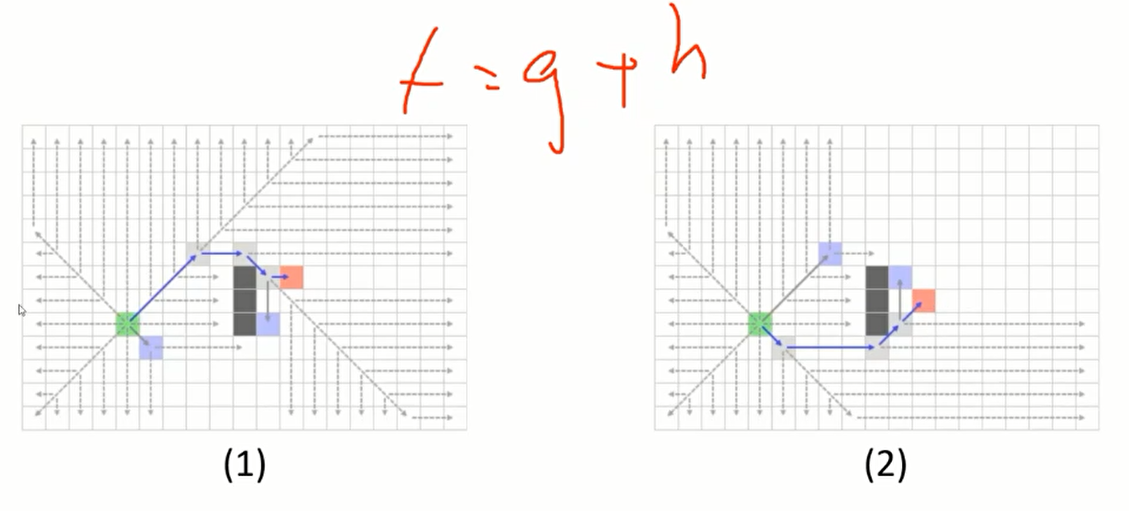
A*出错原因与保证最优性的条件
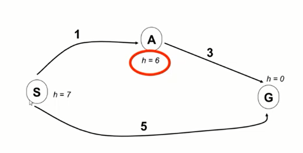
如上图所示,会出现错误。
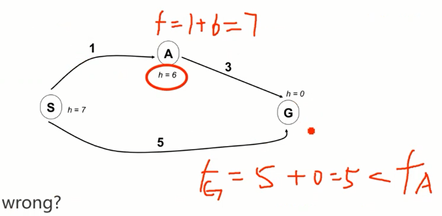
What went wrong?
- For node A: actual least cost to goal (i.e. goal cost) < estimated least cost to goal (i.e. heuristic)
原因在于:A点估计的代价大于实际代价 - We need the estimate to be less than actual least cost to goal (i.e. goal cost) for all nodes!
必须保证每个点的估计代价都低于真实代价,才能保证A*算法的最优性。
Admissible Heuristics
容许的启发函数设计
A Heuristic h is admissible (optimistic) if:
- h(n) <= h*(n) for all node "n", where h*(n) is the true least cost to goal from node "n"
- If the heuristic is admissible, the A* search is optimal
当启发函数满足此条件时,可保证A*算法的最优性 - Coming up with admissible heuristics is most of what's involved in using A* in practice.
提出可行的启发函数是实际使用A*算法的最重要工作。
Example:
An admissible heuristic function has to be designed case by case.
Is Euclidean distance (L2 norm,L2范数) admissible? Always
Is Manhattan distance (L1 norm,L1范数) admissible? Depends
如果机器人允许沿对角线运动,那么Manhattan距离就会大于实际距离。
Is \(L\infty\) norm(\(L\infty\)范数,x向量各个元素绝对值最大那个元素的绝对值) distance admissible? Always
Is 0 distance admissible? Always,退化为Dijkstra算法
Dijkstra vs A*
Sub-optimal Solution and Weighted A*
次优解
What if we intend to use an over-estimate heuristic?
如果刻意地选用过高的启发函数值会怎样?
可以认为此时A*算法在向贪心算法演变。
会得到次优解,但可提升速度。
称之为Weighted A*(权重A*)。
Weighted A*:Expands states based on \(f=g+\epsilon,\epsilon>1\) bias towards states that are closer to goal.
\(\epsilon\)表示有多少的权重直接向目标靠近。
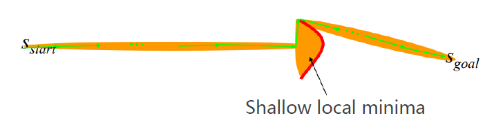
\(\epsilon\)值会决定所规划的轨迹是接近于A*所得出的轨迹,还是贪心算法得出的轨迹(Local Minima)。
- Optimality vs. speed
权衡最优性与速度 - \(\epsilon\)-suboptimal: cost(solution) <= \(\epsilon\) cost (optimal solution)
其cost满足上面的关系 - It can be orders of magnitude faster than A*
比A*的速度可能快几个数量级
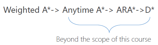
后面三个是几个更新的演进版本
Engineering Considerations
工程上的注意
How to represent grids as graphs?
Each cell is a node. Edges connect adjacent cells.
每个单元格都是一个节点。边连接相邻的单元格。
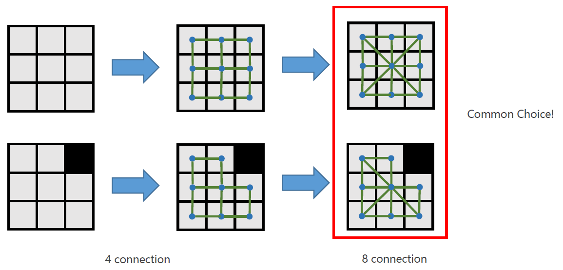
常用的4连通与8连通(8连通是比较常见的)。
三维情况下8连通会变成26连通。
Create a dense graph.
Link the occupancy status stored in the grid map.
Neighbors discovered by grid index.
Perform A* search.
执行碰撞检测时,只需检测相应的grid有没有障碍物。
Priority queue in C++
- std::priority_queue(优先级队列)
- std:make_heap
- std:multimap
The Best Heuristic
假设机器人可以沿着对角线运动,则:

以欧式距离为例,
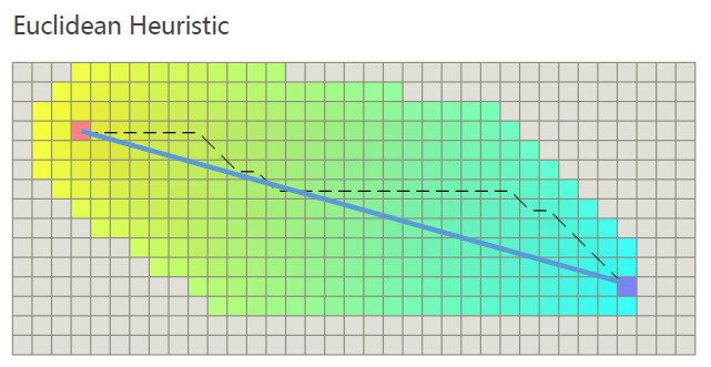
虽然找到了最优路径,但是其效率非常低下(搜索扩展区域很大)。
Why so many nodes expanded?
Because Euclidean distance is far from the truly theoretical optimal solution.
They are useful, but none of them is the best choice, why?
Because none of them is tight.
tight表示其与真实值较为接近。
Tight means who close they measure the true shortest distance.
How to get the truly theoretical optimal solution?
Fortunately, the grid map is highly structural.
对于非常结构化的地图(如栅格地图),以及有结构化的移动规则(如只能左右、上下以及对角线),对于其两点间的最短路径,是可以理论的计算出来的,而无需进行图搜索。
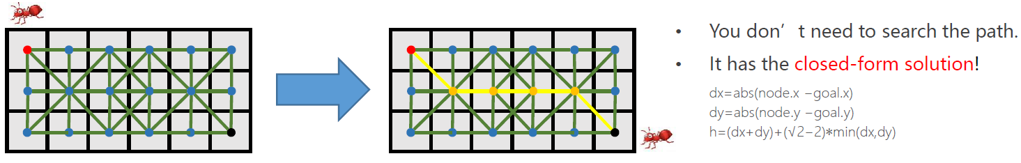
这是一种最紧的Heuristic,称之为Diagonal Heuristic(对角线启发值)。
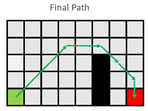
利用这种启发式函数,可以得出最优路径(下图形状不同但长度相同)
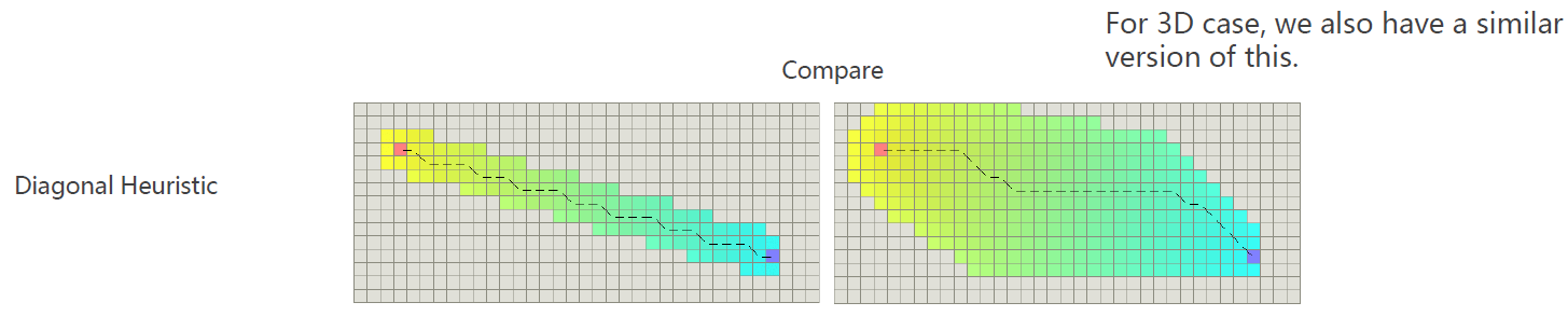
左右两图的算法性能可差距20-50倍。
Tie Breaker
打破平衡环境
原因:path具有对称性(长度一样,但形状不一样)。
- Many paths have the same f value.
- No differences among them making them explored by A* equally.
对于很多节点来说,其具有相同f的节点是无法区分的(不知道选择哪个节点),只能按照先后顺序加入,并均扩展。
这是低效的原因。
效果对比:
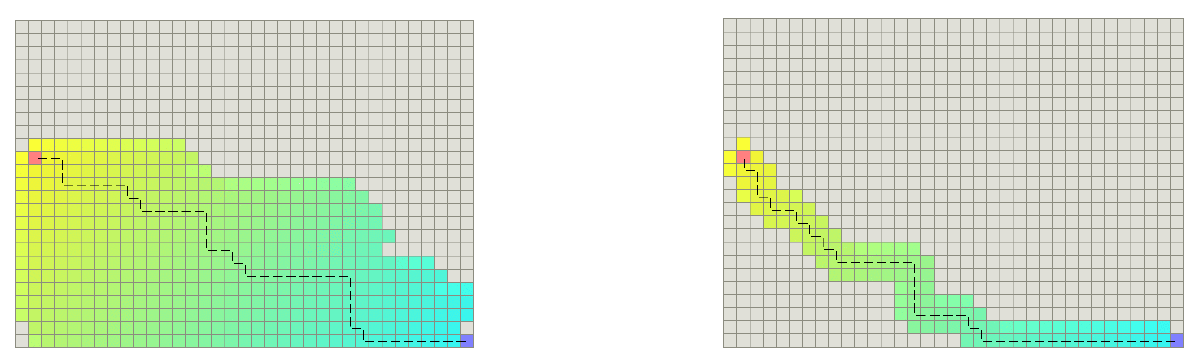
左侧未打破对称性。
出现显著的性能差异(右侧算法效率明显高于左侧)。
介绍第一种方法:
- Manipulate the f value breaks the tie.
修改f值解决这种平衡。 - Make same f values differ.
- Interfere h slightly.
稍微修改h。
minimum cost of one step:单步最小的cost
expected maximum path cost:由于地图大小限制决定的最长路径cost
Slightly breaks the admissibility of h, does it matter?
注意:这种方法(可能)轻微的打破了h的容许性(例如在对角线启发值中,\(h=h^*\)),对其轻微放大,其会不满足容许性。
但在真正的环境中,一般并不影响。
第二种方法:
Core idea of tie breaker:
-
Find a preference among same cost paths
在两个同cost的路径中找到一种倾向性 -
When nodes having same f, compare their h
第一种做法是,在f相等的基础上,对其h进行排序,将h小的放在前面 -
Add deterministic random numbers to the heuristic or edge costs (A hash of the coordinates).
第二种做法是,给每个f加上一个确定性随机数(确定性是指此值不是在运行中确定的,而是根据其坐标值在一开始就确定的,如坐标的哈希值)
此方法实现较为复杂,不推荐使用,但在工程上可能收获更好的效果 -
Prefer paths that are along the straight line from the starting point to the goal.
期望选择靠近起点终点直接连线的路径。
dx1 = abs(node.x -goal.x)
dy1 = abs(node.y -goal.y)
dx2 = abs(start.x-goal.x)
dy2 =abs(start.y -goal.y)
cross = abs(dx1 x dy2-dx2 x dy1)
h=h+ cross × 0.001
-
...Many customized ways
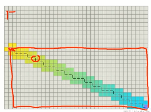
在使用倾向于起终点直线的Tie Breaker时:
Prefer paths that are along the straight line from the starting point to the goal.

其获得的路径并不符合人的直观预期。
另外,连续光滑的曲线路径更适合于机器人的执行。
上面是一些朴素的、工程上的打破Tie Breaker的方法。
注意,不打破Tie并不影响结果的最优性,但会影响算法性能。
因此,引入a systematic approach: Jump Point Search (JPS)。
系统化的实现Tie Breaker的方法。
更高等级的图搜索方法。
Jump Point Search (JPS)
Algorithm Workflow
Core idea of JPS
- Find symmetry and break them.
Compare with A*
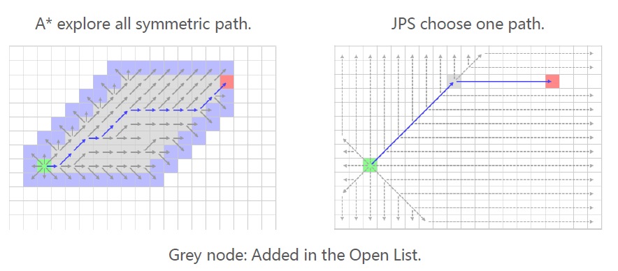
A*算法不具备打破对称性的能力,会探索所有对称路径。
JPS只选择一条路径探索。
JPS explores intelligently, because it always looks ahead based on a rule.
JPS明智地进行探索,因为它总是根据规则向前看。
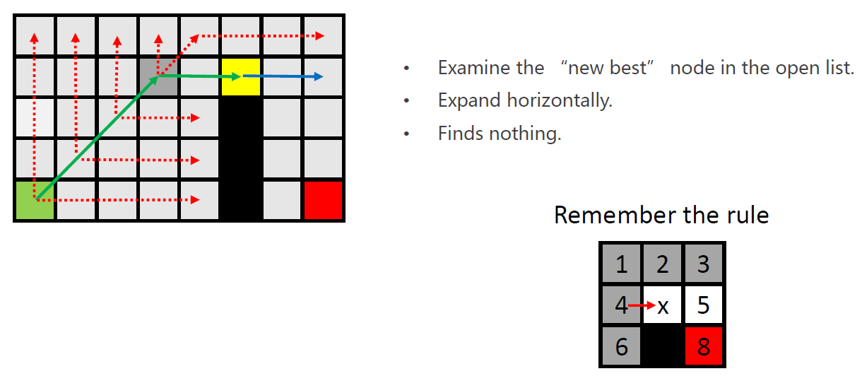
Look Ahead Rule
无障碍物环境
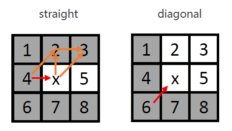
以左图为例,JPS会考量是否有必要通过x点再到达其他节点,准则是通过x再到达其他节点能否降低cost。
若不能,JPS不会将这些节点加入容器。
当面临对称性问题时,如x的父节点4到3,是\(\sqrt{2}+1\)(先通过2再到3),而由父节点必须通过x到达的话,也是\(\sqrt{2}+1\)(4先通过x再到3)。此时,也不会考虑该节点。因此,可打破对称性。
Gray nodes: inferior neighbors, when going to them, the path without x is cheaper. Discard.
灰色:表示劣性节点。当不经过x时代价更低,不考虑。
White nodes: natural neighbors.
白色:表示可考虑的节点。
We only need to consider natural neighbors when expand the search.
左图表示直线运动的情况,右图表示沿对角线运动的情况。
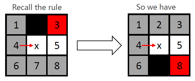
存在障碍物情况
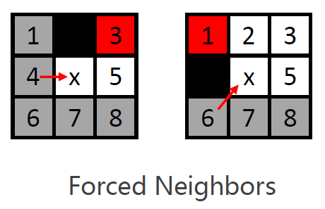
当存在障碍物时,要引入Forced Neighbors(强制节点)。
例如左图的3设置为强制节点。
原因在于,原来3的更短路径(4-2-3)被障碍物中断,3没有更短的路径了。
- There is obstacle adjacent to x
x附近有障碍物。 - Red nodes are forced neighbors.
- A cheaper path from x's parent to them is blocked by obstacle.
从x的父节点出发的更短路径被障碍物中断。
Jumping Rule
-
Recursively apply straight pruning rule (Look Ahead Rule) and identify y as a jump point successor of x. This node is interesting because it has a neighbor z that cannot be reached optimally except by a path that visits x then y
迭代地执行直线的pruning rule(也即Look Ahead Rule的straight),直到到达y节点。原因是y节点拥有Forced Neighbor z,是一个关键节点。跳跃要停止。
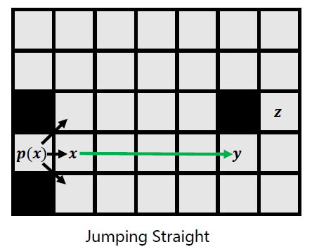
类似地,也有对角线跳跃的规则,但对任何节点,均首先考虑直线跳跃。 -
Recursively apply the diagonal pruning rule and identify y as a jump point successor of x
-
Before each diagonal step we first recurse straight. Only if both straight recursions fail to identify a jump point do we step diagonally again.
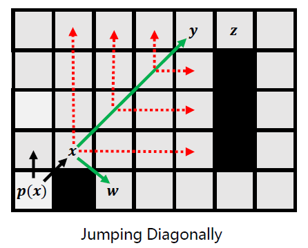
例如,x向右跳跃,最后停在障碍物上,认为跳跃失败。
随后,x向上跳跃,最后停在边界上,也认为跳跃失败。
跳跃失败的原因是,这些路径上不存在所关心的节点。
随后,进行对角线跳跃。
对角线跳跃到y后,在进行水平跳跃,会到达z。
z是一个关键节点,其具有Forced Neighbor(在z的右下角)。
注意,当z为关键节点之后,会返回至y,并将y也标记为关键节点。
关键节点会加入priority queue(优先队列,也即open-list)。 -
Node w, a forced neighbor of x, is expanded as normal. (also push into the open list, the priority queue)
但是,x节点的扩展还未结束,向右下对角线扩展时,会发现Forced Neighbor w。
w也会加入open-list。
至此,x节点的扩展结束,x节点从open-list弹出,并加入close-list。
以上是一次JPS的循环过程。
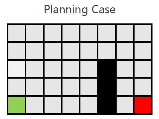
Example of JPS
- Expand horizontally and vertically.
首先进行水平方向与垂直方向的扩展。 - Both jumps end in obstacles.
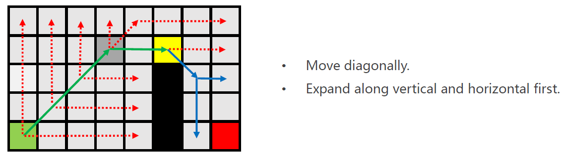
如果两次扩展均以碰到障碍物/边界结束, - Move diagonally.
进行一步的对角线移动。
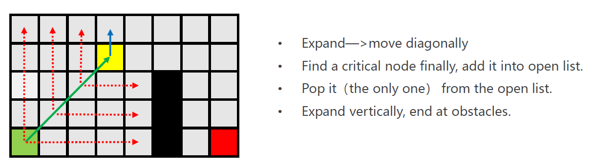
直到:
- Remember: you can only jump straight or diagonally; never piecewise jump
只能进行直线或对角线(也是直线)的跳跃,不能进行折线跳跃。 - Vertically expansion end in obstacle.
- Right-ward expansion finds a node with a forced neighbor.
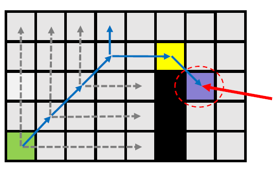
此时,紫色节点是黄色节点的Forced Neighbor。
由于不能进行折线跳跃,因此,回溯到黄色节点左侧两个位置的点,将回溯到的点加入open-list。
意味着从绿色节点开始的一次跳跃,终于找到了其后继点,也即蓝色节点。
绿色节点会从open-list删除,并加入close-list。
- Maintain a priority queue to store all the nodes to be expanded
- The heuristic function h(n) for all nodes are pre-defined
- The priority queue is initialized with the start state \(X_s\)
- Assign \(g(X_s)=0\), and g(n)=infinite for all other nodes in the graph
- Loop
- If the queue is empty, return FALSE; break
- Remove the node "n" with the lowest f(n)=g(n)+h(n) from the priority queue
- Mark node "n" as expanded
- If the node "n" is the goal state, return TRUE;break;
- For all unexpanded neighbors "m" of node "n"
如何寻找unexpanded neighbors是最为重要的问题
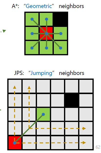
A*直接寻找几何上的邻居
而JPS通过所定义的规则,寻找下一个所跳跃到的后继节点
可以理解为,A*始终寻找几何上紧密连接的邻居,而JPS可在地图的空旷区域进行大规模跳跃- If g(m) = infinite
- g(m)=g(n) +Cnm
- Push node "m" into the queue
- If g(m) > g(n) +Cnm
- g(m)=g(n) +Cnm
- If g(m) = infinite
- end
- End Loop
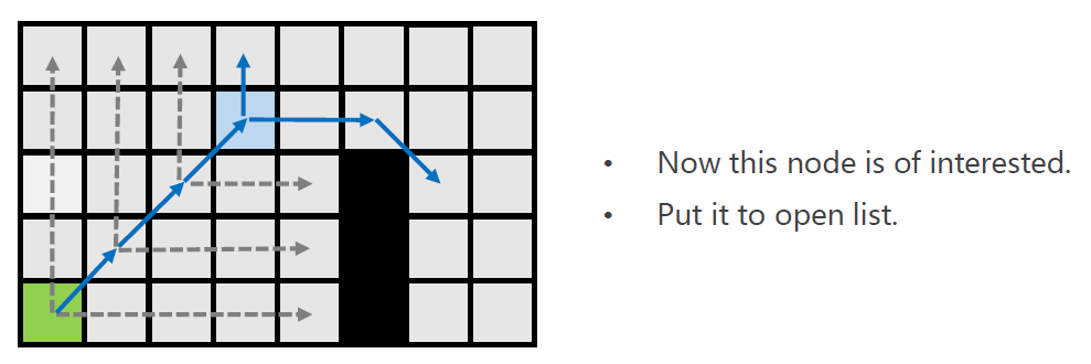
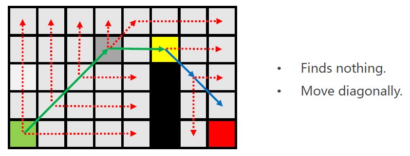
Example

需要注意的是,紫色节点会被加入open-list,原因是发现特殊节点(蓝色)。
但是黄色节点并未从open-list弹出,因为其仅进行了水平方向的扩展,还未进行垂直与对角线方向的扩展。
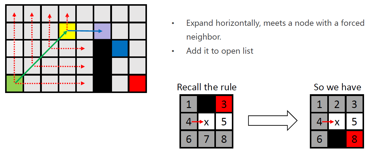
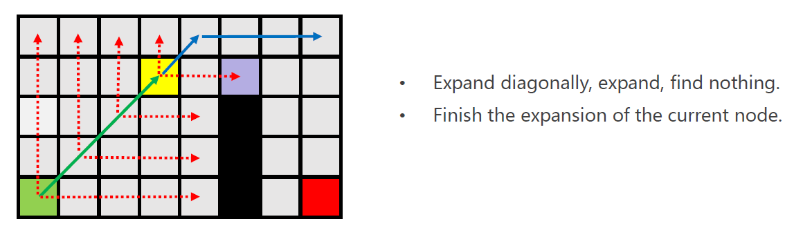
需要进行对角线扩展(仅一步),扩展后再次进行水平与垂直方向的扩展,未发现关键节点。
此时,黄色节点从open-list弹出,并加入close-list。
此时,对黄色节点进行扩展。
由规则可知,没有必要对灰色部分进行扩展。
- Expand horizontally and vertically.
- Finds the goal. Equally interested as finding a node with a forced neighbor
注意:发现目标点,等同于发现Forced Neighbor - Add this node to open list.
将紫色点加入open-list。 - Finish the expand of the current node (No naturally neighbors left).
黄色点结束扩展。 - Pop it out of the open list.
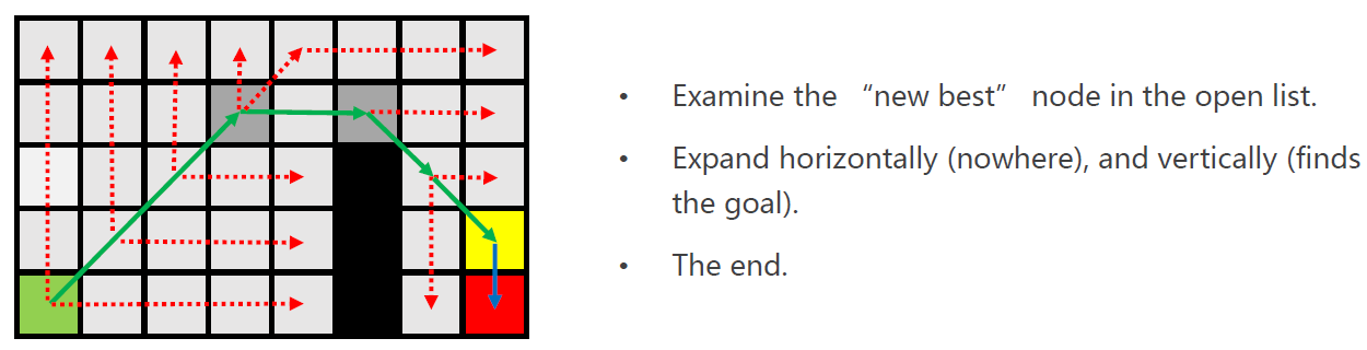
搜索结束。
h值带来的影响:
两条路径的不同原因在于终点位置不同所导致的h值不同。
交互网站:https://zerowidth.com/2013/a-visual-explanation-of-jump-point-search.html
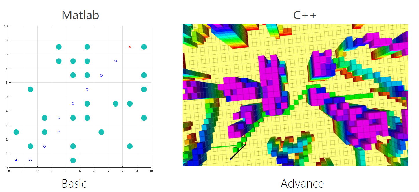
Extension
3D JPS
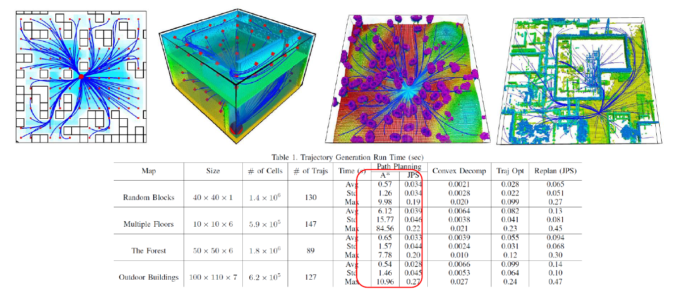
Planning Dynamically Feasible Trajectories for Quadrotors using Safe Flight Corridors in 3-D Complex Environments,
Sikang Liu, RAL 2017
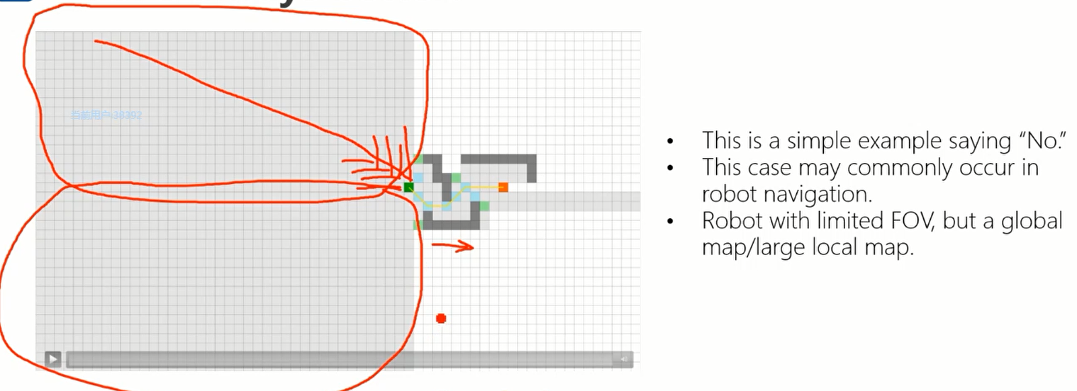
Is JPS always better?
Maze-like environments
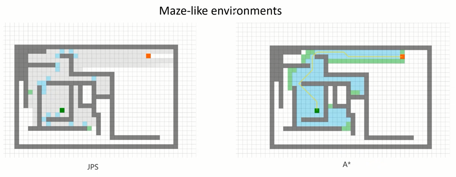
迷宫环境中JPS往往优于A*
而对于机器人来说,往往预先构建了一个非常庞大的地图,但由于机器人只有非常有限的视角(传感器范围有限),可能JPS会比A*慢很多。
Conclusion:
- Most time, especially in complex environments, JPS is better, but far away from "always". Why?
在很多情况尤其是复杂环境下,JPS可以获得更好的结果。 - JPS reduces the number of nodes in Open List, but increases the number of status query.
JPS减少了加入open-list的节点数量,但是增加了对环境的状态查询的次数。空旷空间越大时,越不理想。 - You can try JPS in Homework 2.
- JPS's limitation: only applicable to uniform grid map.
只适用于均匀图(边权值均等),不适用于不同的权重的图。
Homework

 浙公网安备 33010602011771号