


1. EXPLAIN statement
Syntax:
EXPLAIN [FORMATTED|EXTENDED|DEPENDENCY|AUTHORIZATION] hql_query
Aegument description:
- FORMATTED : This provides a formatted JSON version of the query plan.
- EXTENDED : This provides additional information for the operators in the plan,such as file pathname.
- DEPENDENCY : This provides a JSON format output that contains a list of tables and partitions that the query depends on. It has been available since Hive v0.10.0
- AUTHORIZATION : This lists all entities needed to be authorized, including input and output to run the query, and authorization failure, if any. It has been available since Hive v0.14.0.
A typical query plan contains the following three sections. We will also have a look at an example later:
- Abstract Syntax Tree (AST): Hive uses a parser generator called ANTLR (see http:/ / www. antlr. org/ ) to automatically generate a tree syntax for HQL
- Stage Dependencies: This lists all dependencies and the number of stages used to run the query
- Stage Plans: It contains important information, such as operators and sort orders, for running the job
2. ANALYZE statement
Hive statistics are a collection of data that describes more details, such as the number of rows, number of files, and raw data size of the objects in the database. Statistics are the metadata of data, collected and stored in the metastore database. Hive supports statistics at the table, partition, and column level. These statistics serve as an input to the Hive Cost-Based Optimizer (CBO), which is an optimizer used to pick the query plan with the lowest cost in terms of system resources required to complete the query. The statistics are partially gathered automatically in Hive v3.2.0 through to JIRA HIVE-11160 ( https://issues. apache. org/ jira/ browse/ HIVE- 11160 ) or manually through the ANALYZE statement on tables, partitions, and columns, as in the following examples:
2.1 Collect statistics on the existing table.
When the NOSCAN option is specified, the command runs faster by ignoring file scanning but only collecting the number of files and their size
>ANALYZE TABLE employee COMPUTE STATISTICS;
No rows affected (27.979 seconds)
> ANALYZE TABLE employee COMPUTE STATISTICS NOSCAN;
No rows affected (25.979 seconds)
2.2 Collect statistics on specific or all existing partitions
-- Applies for specific partition
> ANALYZE TABLE employee_partitioned PARTITION(year=2018, month=12) COMPUTE STATISTICS;
No rows affected (45.054 seconds)

-- Applies for all partitions
> ANALYZE TABLE employee_partitioned PARTITION(year, month) COMPUTE STATISTICS;
No rows affected (45.054 seconds)
2.3 Collect statistics on columns for existing tables
> ANALYZE TABLE employee_id COMPUTE STATISTICS FOR COLUMNS employee_id;
No rows affected (41.074 seconds)
We can enable automatic gathering of statistics by specifying SET hive.stats.autogather=true . For new tables or partitions that are populated through the INSERT OVERWRITE/INTO statement (rather than the LOAD statement), statistics are automatically collected in the metastore .
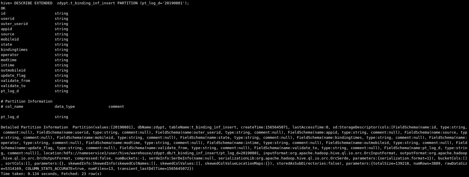
Once the statistics are built and collected, we can check the statistics with the DESCRIBE EXTENDED/FORMATTED statement. From the table/partition output, we can find the statistical information inside the parameters, such as parameters:{numFiles=1, COLUMN_STATS_ACCURATE=true, transient_lastDdlTime=1417726247, numRows=4, totalSize=227, rawDataSize=223}) . The following is an example of checking statistics in a table:
-- Check statistics in a table
> DESCRIBE EXTENDED t_binding_inf_insert;

-- Check statistics in a partition
> DESCRIBE EXTENDED t_binding_inf_insert PARTITION (pt_log_d='20190801');
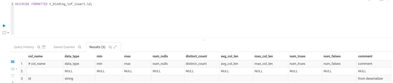
-- Check statistics in a column
> DESCRIBE FORMATTED t_binding_inf_insert.id;
3. Logs
Logs provide detailed information to find out how a query/job runs. By checking the log details, we can identify runtime problems and issues that may cause bad performance. There are two types of log available, the system log and job log.
The system log contains the Hive running status and issues. It is configured in {HIVE_HOME}/conf/hive-log4j.properties . The following three lines of the log properties can be found in the file:
# set logger level
hive.root.logger=WARN,DRFA
# set log file path
hive.log.dir=/tmp/${user.name}
# set log file name
hive.log.file=hive.log
To modify the logger level, we can either modify the preceding property file that applies to all users, or set a Hive command-line config that only applies to the current user session, such as:
$hive --hiveconf hive.root.logger=DEBUG,console
The job log contains job information and is usually managed by Yarn. To check a job log, use
yarn logs -applicationId <application_id>
4.Using Index
Using indexes is a very common best practice for performance tuning in relational databases. Hive has supported index creation on tables/partitions since Hive v0.7.0. An index in Hive provides a key-based data view and better data access for certain operations,such as WHERE , GROUP BY , and JOIN . Using an index is always a cheaper alternative than full-table scans. The command to create an index in HQL is straightforward, as follows:
CREATE INDEX idx_id_employee_id
ON TABLE employee_id (employee_id)
AS 'COMPACT'
WITH DEFERRED REBUILD;
No rows affected (1.149 seconds)
In addition to this COMPACT index, which stores the pair of the indexed column's value and its block ID, HQL has also supported BITMAP indexes since v0.8.0 for column values with less variance, as shown in the following example:
CREATE INDEX idx_gender_employee_id
ON TABLE employee_id (gender_age)
AS 'BITMAP'
WITH DEFERRED REBUILD;
No rows affected (0.251 seconds)
The WITH DEFERRED REBUILD option in this example prevents the index from immediately being built. To build the index, we can issue the ALTER...REBUILD commands as shown in the following example. When data in the base table changes, the same command must be used again to bring the index up to date. This is an atomic operation. If the index rebuilt on a table has been previously indexed failed, the state of the index remains the same. See this example to build the index:
>ALTER INDEX idx_id_employee_id ON employee_id REBUILD;
No rows affected (111.413 seconds)
> ALTER INDEX idx_gender_employee_id ON employee_id REBUILD;
No rows affected (82.23 seconds)
Once the index is built, a new index table is created for each index with the name in the format of <database_name>__<table_name>_<index_name>__ :
> SHOW TABLES '*idx*';
+-----------+---------------------------------------------+-----------+
|TABLE_SCHEM|TABLE_NAME                                   | TABLE_TYPE|
+-----------+---------------------------------------------+-----------+
|default    |default__employee_id_idx_id_employee_id__    |INDEX_TABLE|
|default    |default__employee_id_idx_gender_employee_id__|INDEX_TABLE|
+-----------+---------------------------------------------+-----------+
The index table contains the indexed column, the _bucketname (a typical file URI on HDFS), and _offsets (offsets for each row). Then, this index table can be referred to when we query the indexed columns from the indexed table, as shown here:
> DESC default__employee_id_idx_id_employee_id__;
+--------------+----------------+----------+
|
col_name      |data_type      |comment|
+--------------+----------------+----------+
| employee_id | int           |       |
| _bucketname | string        |       |
| _offsets    | array<bigint> |       |
+--------------+----------------+----------+
3 rows selected (0.135 seconds)
> SELECT * FROM default__employee_id_idx_id_employee_id__;
+--------------+------------------------------------------------------+
| employee_id | _bucketname                              | _offsets |
+--------------+------------------------------------------------------+
| 100         | .../warehouse/employee_id/employee_id.txt | [0]     |
| 101         | .../warehouse/employee_id/employee_id.txt | [66]    |
| 102         | .../warehouse/employee_id/employee_id.txt | [123]   |
+--------------+-------------------------------------------+----------+
3 rows selected (0.219 seconds)
To drop an index, we can only use the DROP INDEX index_name ON table_name statement as follows. We cannot drop the index with a DROP TABLE statement:
> DROP INDEX idx_gender_employee_id ON employee_id;
No rows affected (0.247 seconds)
5. Use skewed/temporary tables
Besides regular internal/external or partition tables, we should also consider using a skewed or temporary table for better design as well as performance.
Since Hive v0.10.0, HQL has supported the creation of a special table for organizing skewed data. A skewed table can be used to improve performance by splitting those skewed values into separate files or directories automatically. As a result, the total number of files or partition folders is reduced. Also, a query can include or ignore this data quickly and efficiently. Here is an example used to create a skewed table:
CREATE TABLE sample_skewed_table (
dept_no int,
dept_name string
)
SKEWED BY (dept_no) ON (1000, 2000); -- Specify value skewed


DESC FORMATTED sample_skewed_table;
+-----------------+------------------+---------+
| col_name        | data_type        | comment |
+-----------------+------------------+---------+
| ...             | ...              |         |
| Skewed Columns: | [dept_no]        | NULL    |
| Skewed Values:  | [[1000], [2000]] | NULL    |
| ...             | ...              |         |
+-----------------+------------------+---------+
On the other hand, using temporary tables in HQL to keep intermediate data during data recursive processing will save you the effort of rebuilding the common or shared result set. In addition, temporary tables can leverage storage policy settings to use SSD or memory for data storage, and this adds up to better performance too.
6. Storage Optimization
6.1 File Format
Hive supports TEXTFILE , SEQUENCEFILE , AVRO , RCFILE , ORC , and PARQUET file formats.There are two HQL statements used to specify the file format as follows:
CREATE TABLE ... STORE AS <file_format>                                  --Specify the file format when creating a table
ALTER TABLE ... [PARTITION partition_spec] SET FILEFORMAT <file_format>  --Modify the file format (definition only) in an existing table
Once a table stored in text format is created, we can load text data directly into it. To load text data into tables that have other file formats, we can first load the data into a table stored as text, where we use INSERT OVERWRITE/INTO TABLE ... SELECT to select data from it and then insert the data into the tables that have other file formats.
To change the default file format for table creation, we can
set the hive.default.fileformat = <file_format> property for all tables
or hive.default.fileformat.managed = <file_format> only for internal/managed tables.
TEXT , SEQUENCE , and AVRO files as a row-oriented file storage format are not optimal solutions since the query has to read a full row even if only one column is being requested. On the other hand, a hybrid row-columnar storage file format, such as RCFILE , ORC ,or PARQUET , is used to resolve this problem. The details of file formats supported by HQL are as follows:
- TEXTFILE : This is the default file format for table creation. Data is stored in clear text for this format. A text file is naturally splittable and able to be processed in parallel. It can also be compressed with algorithms, such as GZip, LZO, and Snappy. However, most compressed files are not splittable for parallel processing. As a result, they use only one job with a single mapper to process data slowly. The best practice for using compressed text files is to make sure the file is not too big and close to a couple of HDFS block sizes.
- SEQUENCEFILE : This is a binary storage format for key/value pairs. The benefit of a sequence file is that it is more compact than a text file and fits well with the MapReduce output format. Sequence files can be compressed to record or block level, where the block level has a better compression ratio. To enable block-level compression, we need use do the following settings: set hive.exec.compress.output=true; and set io.seqfile.compression.type=BLOCK;
- AVRO : This is also a binary format. More than that, it is also a serialization and deserialization framework. AVRO provides a data schema that describes the data structure and also handles the schema changes, such as adding, renaming, and removing columns. The schema is stored along with data for any further processing. Considering AVRO 's advantages for dealing with schema evolution, it is recommended to use it when mapping the source data, which is likely to have schema changes time by time.
- RCFILE : This is short for Record Columnar File. It is a flat file consisting of binary key/value pairs that share many similarities with a sequence file. The RCFile splits data horizontally into row groups. One or several groups are stored in an HDFS file. Then, RCFile saves the row group data in a columnar format by saving the first column across all rows, then the second column across all rows, and so on. This format is splittable and allows Hive to skip irrelevant parts of the data and get the results faster and cheaper.
- ORC : This is short for Optimized Row Columnar. It has been available since Hive v0.11.0. The ORC format can be considered an improved version of RCFILE . It provides a larger block size of 256 MB by default ( RCFILE has 4 MB and SEQUENCEFILE has 1 MB), optimized for large sequential reads on HDFS for more throughput and fewer files to reduce overload in the namenode. Different from RCFILE , which relies on the metastore to know data types, the ORC file understands the data types by using specific encoders so that it can optimize compression depending on different types. It also stores basic statistics, such as MIN , MAX , SUM , and COUNT , on columns as well as a lightweight index that can be used to skip blocks of rows that do not matter.
- PARQUET : This is another row columnar file format that has a similar design to that of ORC . What's more, Parquet has a wider range of support for the majority of projects in the ecosystem, compared to ORC which is mainly supported by Hive, Pig, and Spark. PARQUET leverages the best practices in the design of Google's Dremel (see http:/ / research. google. com/ pubs/ pub36632. html ) to support the nested structure of data. PARQUET has been supported by a plugin since Hive v0.10.0 and got native support after v0.13.0.
Depending on the technology stacks being used, it is suggested to use the ORC format if Hive is the majority tool used to define or process data. If you use several tools in the ecosystem, PARQUET is the better choice in terms of adaptability.
6.2 Compression
Compression techniques in Hive can significantly reduce the amount of data transferring between mappers and reducers by properly compressing intermediate and final output data. As a result, the query will have better performance. To compress intermediate files produced between multiple MapReduce jobs, we need to set the following property ( false by default) in the command-line session or the hive-site.xml file:
SET hive.exec.compress.intermediate=true;
Then, we need to decide which compression codec to configure. A list of commonly supported codecs is in the following table:
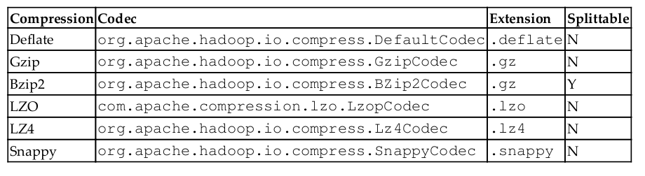
Deflate ( .deflate ) is a default codec with a balanced compression ratio and CPU cost.
The compression ratio for Gzip is very high, as is its CPU cost.
Bzip2 is splittable, but it is too slow for compression considering its huge CPU cost, like Gzip.
LZO files are not natively splittable, but we can preprocess them (using com.hadoop.compression.lzo.LzoIndexer ) to create an index that determines the file splits. When it comes to the balance of CPU cost and compression ratio,
LZ4 or Snappy do a better job than Deflate, but Snappy is more popular. Since the majority of compressed files are not splittable, it is not suggested to compress a single big file. The best practice is to produce compressed files in a couple of HDFS block sizes so that each file takes less time for processing. The compression codec can be specified in either mapred-site.xml , hive- site.xml , or a command-line session as follows:
SET hive.intermediate.compression.codec=org.apache.hadoop.io.compress.SnappyCodec;
Intermediate compression will only save disk space for specific jobs that require multiple MapReduce jobs. For further saving of disk space, the actual Hive output files can be compressed. When the hive.exec.compress.output property is set to true , Hive will use the codec configured by the mapreduce.output.fileoutputformat.compress.codec property to compress the data in HDFS as follows. These properties can be set in the hive-site.xml or in the command-line session:
SET hive.exec.compress.output=true;
SET mapreduce.output.fileoutputformat.compress.codec=org.apache.hadoop.io.compress.SnappyCodec;
6.3 Storage optimization
Data that is used or scanned frequently can be identified as hot data. Usually, query performance on hot data is critical for overall performance. Increasing the data replication factor in HDFS (see the following example) for hot data could increase the chance of data being hit locally by jobs and improve the overall performance. However, this is a trade-off against storage:
$ hdfs dfs -setrep -R -w 4 /user/hive/warehouse/employee
Replication 4 set: /user/hive/warehouse/employee/000000_0
On the other hand, too many files or redundancy could make namenode's memory exhausted, especially lots of small files whose sizes are less than the HDFS block sizes. Hadoop itself already has some solutions to deal with many small-file issues in the following ways:
- Hadoop Archive/ HAR : These are toolkits to pack small files introduced before.
- SEQUENCEFILE Format: This is a format that can be used to compress small files into bigger files.
- CombineFileInputFormat : A type of InputFormat to combine small files before map and reduce processing. It is the default InputFormat for Hive (see https://issues.apache.org/jira/browse/HIVE-2245).
- HDFS Federation: It supports multiple namenodes to manage more files.
We can also leverage other tools in the Hadoop ecosystem if we have them installed, such as the following:
- HBase has a smaller block size and better file format to deal with smaller file storage and access issues.
- Flume NG can be used as a pipe to merge small files into big ones.
- Developed and scheduled a file merge program to merge small files in HDFS or before loading the files to HDFS
For Hive, we can use the following configurations to merge files of query results and avoid recreating small files:
- hive.merge.mapfiles : This merges small files at the end of a map-only job. By default, it is true .
- hive.merge.mapredfiles : This merges small files at the end of a MapReduce job. Set it to true, as the default is false .
- hive.merge.size.per.task : This defines the size of merged files at the end of the job. The default value is 256,000,000.
- hive.merge.smallfiles.avgsize : This is the threshold for triggering file merge. The default value is 16,000,000.
When the average output file size of a job is less than the value specified by the hive.merge.smallfiles.avgsize property and both hive.merge.mapfiles (for map-only jobs) and hive.merge.mapredfiles (for MapReduce jobs) are set to true, Hive will start an additional MapReduce job to merge the output files into big files.
--every map split size
set mapred.max.split.size=256000000;
--min split size for single node
set mapred.min.split.size.per.node=100000000;
--min split size for single rack
set mapred.min.split.size.per.rack=100000000;
--merge file format
set hive.input.format=org.apache.hadoop.hive.ql.io.CombineHiveInputFormat;

--merge files at the finished time of map only task.
set hive.merge.mapfiles = true;
--merge when MapReduce task finishs.
set hive.merge.mapredfiles = true;
--merge file size
set hive.merge.size.per.task = 256000000;
set hive.merge.smallfiles.avgsize=160000000;
set hive.exec.reducers.bytes.per.reducer= 5120000000;
7. Job optimization
Job optimization covers experience and skills to improve performance in the areas of job-running mode, JVM reuse, job parallel running, and query join optimizations.
7.1 Local mode
Hadoop can run in standalone, pseudo-distributed, and fully distributed mode. Most of the time, we need to configure it to run in fully distributed mode. When the data to process is small, it is an overhead to start distributed data processing since the launch time of the fully distributed mode takes more time than the job processing time. Since v0.7.0, Hive has supported automatic conversion of a job to run in local mode with the following settings:
SET hive.exec.mode.local.auto=true; -- default false
SET hive.exec.mode.local.auto.inputbytes.max=50000000;
SET hive.exec.mode.local.auto.input.files.max=5; -- default 4
A job must satisfy the following conditions to run in local mode:
- The total input size of the job is less than the value set by hive.exec.mode.local.auto.inputbytes.max
- The total number of map tasks is less than the value set by hive.exec.mode.local.auto.input.files.max
- The total number of reduce tasks required is 1 or 0
7.2 JVM reuse
By default, Hadoop launches a new JVM for each map or reduce job and runs the map or reduce task in parallel. When the map or reduce job is a lightweight job running only for a few seconds, the JVM startup process could be a significant overhead. Hadoop has an option to reuse the JVM by sharing the JVM to run mapper/reducer serially instead of in parallel. JVM reuse applies to map or reduce tasks in the same job. Tasks from different jobs will always run in a separate JVM.
To enable reuse, we can set the maximum number of tasks for a single job for JVM reuse using the following property. Its default value is 1. If set to -1, there is no limit:
SET mapreduce.job.jvm.numtasks=5;
7.3 Parallel execution
Hive queries are commonly translated into a number of stages that are executed by the default sequence. These stages are not always dependent on each other. Instead they can run in parallel to reduce the overall job running time. We can enable this feature with the following settings and set the expected number of jobs running in parallel:
SET hive.exec.parallel=true; -- default false
SET hive.exec.parallel.thread.number=16; -- default 8
Parallel execution will increase cluster utilization. If the utilization of a cluster is already very high, parallel execution will not help much in terms of overall performance.
7.4 Join optimization
7.4.1 Common join
The common join is also called the reduce side join. It is a basic join in HQL and works most of the time. For common joins, we need to make sure the big table is on the rightmost side or specified by hit, as follows:
/*+ STREAMTABLE(stream_table_name) */
7.4.2 Map join
Map join is used when one of the join tables is small enough to fit in the memory, so it is fast but limited by the table size. Since Hive v0.7.0, it has been able to convert map join automatically with the following settings:
SET hive.auto.convert.join=true;                            -- default true after v0.11.0
SET hive.mapjoin.smalltable.filesize=600000000;             -- default 25m
SET hive.auto.convert.join.noconditionaltask=true;          -- default value above is true so map join hint is not needed
SET hive.auto.convert.join.noconditionaltask.size=10000000; -- default value above controls the size of table to fit in memory
Once join auto-convert is enabled, Hive will automatically check whether the smaller table file size is bigger than the value specified by hive.mapjoin.smalltable.filesize , and then it will convert the join to a common join. If the file size is smaller than this threshold, it will try to convert the common join into a map join. Once auto-convert join is enabled, there is no need to provide the map join hints in the query.
7.4.3 Bucket map join
A bucket map join is a special type of map join applied on the bucket tables. To enable a bucket map join, we need to enable the following settings:
SET hive.auto.convert.join=true;
SET hive.optimize.bucketmapjoin=true; -- default false
In a bucket map join, all the join tables must be bucket tables and join on bucket columns.
In addition, the bucket number in the bigger tables must be a multiple of the bucket number in the smaller tables.
7.4.4 Sort merge bucket (SMB) join
SMB is a join performed on bucket tables that have the same sorted, bucket, and join condition columns. It reads data from both bucket tables and performs common joins (map and reduce triggered) on the bucket tables. We need to enable the following properties to use SMB:
SET hive.input.format=org.apache.hadoop.hive.ql.io.BucketizedHiveInputFormat;
SET hive.auto.convert.sortmerge.join=true;
SET hive.optimize.bucketmapjoin=true;
SET hive.optimize.bucketmapjoin.sortedmerge=true;
SET hive.auto.convert.sortmerge.join.noconditionaltask=true;
7.4.5 Sort merge bucket map (SMBM) join
An SMBM join is a special bucket join but triggers a map-side join only. It can avoid caching all rows in the memory like a map join does. To perform SMBM joins, the join tables must have the same bucket, sort, and join condition columns.
To enable such joins, we need to enable the following settings:
SET hive.auto.convert.join=true;
SET hive.auto.convert.sortmerge.join=true;
SET hive.optimize.bucketmapjoin=true;
SET hive.optimize.bucketmapjoin.sortedmerge=true;
SET hive.auto.convert.sortmerge.join.noconditionaltask=true;
SET hive.auto.convert.sortmerge.join.bigtable.selection.policy=org.apache.hadoop.hive.ql.optimizer.TableSizeBasedBigTableSelectorForAutoSMJ;
7.5 Job engine
Hive supports running jobs on different engines. The choice of engine will also impact the overall performance. However, this is a bigger change compared to the other settings. Also, this change requires a service restart rather than temporarily make it effective in command- line session. Here is the syntax to set the engine as well as details for each of them:
SET hive.execution.engine=<engine>; -- <engine> = mr|tez|spark
- mr : This is the default engine, MapReduce. It was deprecated after Hive v2.0.0.
- tez : Tez ( http:/ / tez. apache.org/ ) is an application framework built on Yarn that can execute complex Directed Acyclic Graphs (DAGs) for general data- processing tasks. Tez further splits map and reduce jobs into smaller tasks and combines them in a flexible and efficient way for execution. Tez is considered a flexible and powerful successor to the MapReduce framework. Tez is production- ready and being used most of the time to replace the mr engine.
- spark : Spark is another general purpose big data framework. Its component, Spark SQL, supports a subset of HQL and provides similar syntax to HQL. By using Hive over Spark, Hive can leverage Spark's in-memory computing model as well as Hive's mature cost-based optimizer. However, Hive over Spark requires manual configurations and still lacks solid use cases in production. For more details of Hive over Spark, refer to the Wiki page at ( https:/ / cwiki. apache. org/ confluence/ display/ Hive/ Hive+on+Spark%3A+Getting+Started ).
- mr3 : MR3 is another experiment engine ( https:/ / mr3. postech. ac. kr/ ). It is similar to Tez but with the enhancements of simpler design, better performance, and more features. MR3 is documented as ready for production use and supports all major features from Tez, such as Kerberos-based security, authentication and authorization, fault tolerance, and recovery. However, it lacks a solid production use case and best practices in production deployment, as well as CDH or HDP distribution support.
Live Long And Process (LLAP) functionality was added in Hive v2.0.0. It combines a live long running query service and intelligent in-memory caching to deliver fast queries. Together with a job engine, LLAP provides a hybrid execution model to improve overall Hive performance. LLAP needs to work through Apache Slider ( https://slider.incubator.apache.org/) and only works with Tez for now. In the future, it will support other engines. The recent HDP has provided LLAP supported thought Tez.
7.6 Optimizer
Similar to relational databases, Hive generates and optimizes each query's logical and physical execution plan before submitting for final execution. There are two major optimizers now in Hive to further optimize query performance in general, Vectorize and Cost-Based Optimization (CBO).
7.6.1 Vectorization optimization
Vectorization optimization processes a larger batch of data at the same time rather than one row at a time, thus significantly reducing computing overhead.
Each batch consists of a column vector that is usually an array of primitive types. Operations are performed on the entire column vector, which improves the instruction pipelines and cache use. Files must be stored in the ORC format in order to use vectorization. For more details on vectorization, please refer to the Hive Wiki ( https://cwiki.apache.org/confluence/display/Hive/Vectorized+Query+Execution ).
To enable vectorization, we need to use the following setting:
SET hive.vectorized.execution.enabled=true; -- default false
7.6.2 Cost-based optimization
CBO in Hive is powered by Apache Calcite (http://calcite.apache.org/), which is an open source, enterprise-grade cost-based logical optimizer and query execution framework. Hive CBO generates efficient execution plans by examining the query cost, which is collected by ANALYZE statements or the metastore itself, ultimately cutting down on query execution time and reducing resource utilization. To use CBO, set the following properties:
SET hive.cbo.enable=true; -- default true after v0.14.0
SET hive.compute.query.using.stats=true; -- default false
SET hive.stats.fetch.column.stats=true; -- default false
SET hive.stats.fetch.partition.stats=true; -- default true

 浙公网安备 33010602011771号