GBDT + LR
一、理论
GBDT+LR并不是两个模型的结合,而是一种特征的转化。也就是说这个问题我们需要从特征的角度去思考而不是从模型。
GBDT是由多棵回归树组成的森林模型。对于每一个样本,它在预测的时候都会落到每一棵子树的其中一个叶子节点上。这样就可以使用GBDT来进行特征的映射。
所以,GBDT相当于一次embedding。完成了原始特征的映射,映射后的特征作为逻辑回归模型的输入样本。
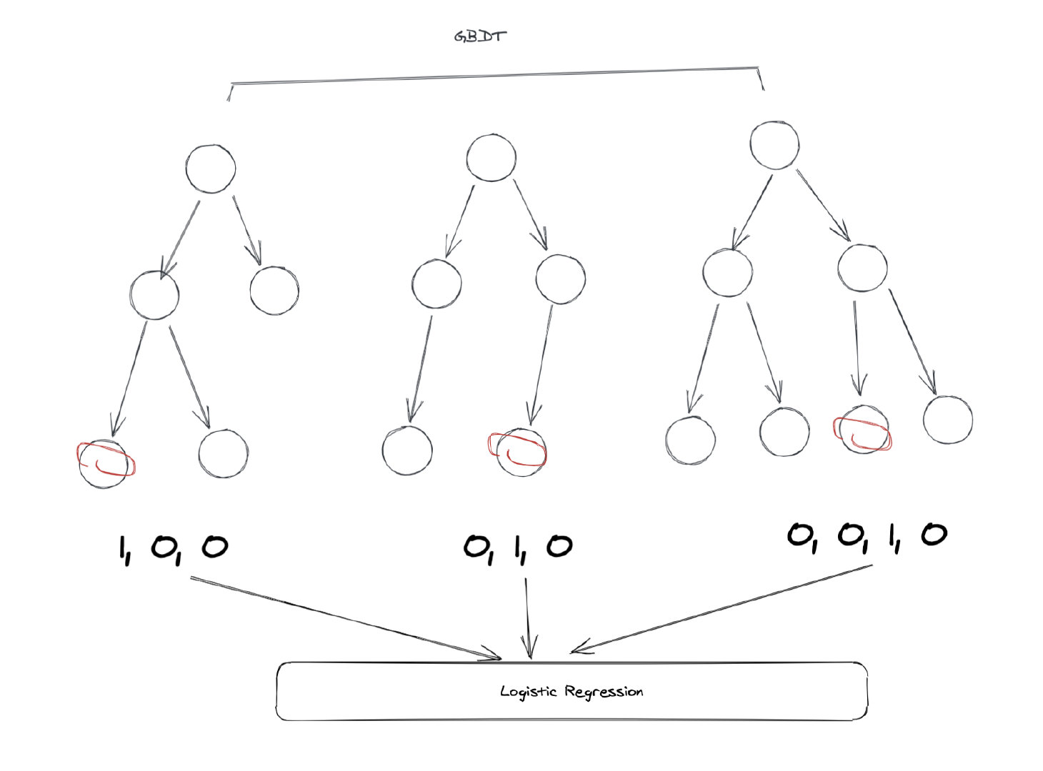
在上图这个例子当中,GBDT一共有3棵子树,第一棵子树有3个叶子节点。我们的样本落到了第一个,所以第一棵子树对应的one-hot结果是[1, 0, 0],第二棵子树也有3个节点,样本落到了第二个节点当中,所以one-hot的结果是[0, 1, 0],同理可以得到第三棵子树的结果是[0, 0, 1, 0]。
最后把这些树的向量合并在一起,就得到了一个新的向量:[1, 0, 0, 0, 1, 0, 0, 0, 1, 0],这个向量就是LR模型的输入。
二、sklearn实现
import numpy as np
np.random.seed(10)
import matplotlib.pyplot as plt
from sklearn.datasets import make_classification
from sklearn.linear_model import LogisticRegression
from sklearn.ensemble import GradientBoostingClassifier
from sklearn.preprocessing import OneHotEncoder
from sklearn.model_selection import train_test_split
from sklearn.metrics import roc_curve


n_estimator = 10
X, y = make_classification(n_samples=80000)
X_train, X_test, y_train, y_test = train_test_split(X, y, test_size=0.5)

# 将训练集切分为两部分,一部分用于训练GBDT模型,另一部分输入到训练好的GBDT模型生成GBDT特征,然后作为LR的特征。这样分成两部分是为了防止过拟合。
X_train, X_train_lr, y_train, y_train_lr = train_test_split(
    X_train, y_train, test_size=0.5)

#print(X_train.shape)  (20000, 20)
#print(y_train.shape) (20000,)

gbdt = GradientBoostingClassifier(n_estimators=n_estimator)

"""
n_estimators,最大的弱学习器的个数,即有多少个回归树
max_depth : int, default=3。每个回归树的的深度
"""


gbdt_enc = OneHotEncoder()
lr = LogisticRegression(max_iter=1000)
gbdt.fit(X_train, y_train) # 训练GBDT模型

gbdt_enc.fit(gbdt.apply(X_train)[:, :, 0]) # one-hot编码,shape=(20000, 80)
# model.apply(X_train)返回训练数据X_train在训练好的模型里每棵树中所处的叶子节点的位置(索引)
lr.fit(gbdt_enc.transform(gbdt.apply(X_train_lr)[:, :, 0]), y_train_lr) # 训练LR模型

y_pred_gbdt_lr = lr.predict_proba(
    gbdt_enc.transform(gbdt.apply(X_test)[:, :, 0]))[:, 1]
print(y_pred_gbdt_lr)
fpr_grd_lr, tpr_grd_lr, _ = roc_curve(y_test, y_pred_gbdt_lr)

plt.figure(1)
plt.plot([0, 1], [0, 1], 'k--')

plt.plot(fpr_grd_lr, tpr_grd_lr, label='GBDT + LR')
plt.xlabel('False positive rate')
plt.ylabel('True positive rate')
plt.title('ROC curve')
plt.legend(loc='best')
plt.show()

plt.figure(2)
plt.xlim(0, 0.2)
plt.ylim(0.8, 1)
plt.plot([0, 1], [0, 1], 'k--')

plt.plot(fpr_grd_lr, tpr_grd_lr, label='GBDT + LR')
plt.xlabel('False positive rate')
plt.ylabel('True positive rate')
plt.title('ROC curve (zoomed in at top left)')
plt.legend(loc='best')
plt.show()

 浙公网安备 33010602011771号