Time series

time series

import pandas as pd

data = pd.read_csv(r'../data/data.csv')

data
# 数据那么好，为什么不回归呢...

	x1	x2	x3	x4	x5	x6	x7	x8	x9	x10	x11	x12	x13	y
0	3831732	181.54	448.19	7571.00	6212.70	6370241	525.71	985.31	60.62	65.66	120.0	1.029	5321	64.87
1	3913824	214.63	549.97	9038.16	7601.73	6467115	618.25	1259.20	73.46	95.46	113.5	1.051	6529	99.75
2	3928907	239.56	686.44	9905.31	8092.82	6560508	638.94	1468.06	81.16	81.16	108.2	1.064	7008	88.11
3	4282130	261.58	802.59	10444.60	8767.98	6664862	656.58	1678.12	85.72	91.70	102.2	1.092	7694	106.07
4	4453911	283.14	904.57	11255.70	9422.33	6741400	758.83	1893.52	88.88	114.61	97.7	1.200	8027	137.32
5	4548852	308.58	1000.69	12018.52	9751.44	6850024	878.26	2139.18	92.85	152.78	98.5	1.198	8549	188.14
6	4962579	348.09	1121.13	13966.53	11349.47	7006896	923.67	2492.74	94.37	170.62	102.8	1.348	9566	219.91
7	5029338	387.81	1248.29	14694.00	11467.35	7125979	978.21	2841.65	97.28	214.53	98.9	1.467	10473	271.91
8	5070216	453.49	1370.68	13380.47	10671.78	7206229	1009.24	3203.96	103.07	202.18	97.6	1.560	11469	269.10
9	5210706	533.55	1494.27	15002.59	11570.58	7251888	1175.17	3758.62	109.91	222.51	100.1	1.456	12360	300.55
10	5407087	598.33	1677.77	16884.16	13120.83	7376720	1348.93	4450.55	117.15	249.01	101.7	1.424	14174	338.45
11	5744550	665.32	1905.84	18287.24	14468.24	7505322	1519.16	5154.23	130.22	303.41	101.5	1.456	16394	408.86
12	5994973	738.97	2199.14	19850.66	15444.93	7607220	1696.38	6081.86	128.51	356.99	102.3	1.438	17881	476.72
13	6236312	877.07	2624.24	22469.22	18951.32	7734787	1863.34	7140.32	149.87	429.36	103.4	1.474	20058	838.99
14	6529045	1005.37	3187.39	25316.72	20835.95	7841695	2105.54	8287.38	169.19	508.84	105.9	1.515	22114	843.14
15	6791495	1118.03	3615.77	27609.59	22820.89	7946154	2659.85	9138.21	172.28	557.74	97.5	1.633	24190	1107.67
16	7110695	1304.48	4476.38	30658.49	25011.61	8061370	3263.57	10748.28	188.57	664.06	103.2	1.638	29549	1399.16
17	7431755	1700.87	5243.03	34438.08	28209.74	8145797	3412.21	12423.44	204.54	710.66	105.5	1.670	34214	1535.14
18	7512997	1969.51	5977.27	38053.52	30490.44	8222969	3758.39	13551.21	213.76	760.49	103.0	1.825	37934	1579.68
19	7599295	2110.78	6882.85	42049.14	33156.83	8323096	4454.55	15420.14	228.46	852.56	102.6	1.906	41972	2088.14

AutoGluon : Regression

train_data_reg = data.iloc[0:-2,:]
test_data_reg = data.iloc[-2:,:]

from autogluon.tabular import TabularDataset, TabularPredictor
train_data_reg_auto = TabularDataset(train_data_reg)
test_data_reg_auto = TabularDataset(test_data_reg)

predictor = TabularPredictor(label='y').fit(train_data=train_data_reg_auto)
predictions = predictor.predict(test_data_reg_auto)
## AutoGluon infers your prediction problem is: 'regression'
## (because dtype of label-column == float and many unique label-values observed).

No path specified. Models will be saved in: "AutogluonModels/ag-20220331_070120\"
Beginning AutoGluon training ...
AutoGluon will save models to "AutogluonModels/ag-20220331_070120\"
AutoGluon Version:  0.4.0
Python Version:     3.9.7
Operating System:   Windows
Train Data Rows:    18
Train Data Columns: 13
Label Column: y
Preprocessing data ...
AutoGluon infers your prediction problem is: 'regression' (because dtype of label-column == float and many unique label-values observed).
	Label info (max, min, mean, stddev): (1535.14, 64.87, 482.99222, 462.62691)
	If 'regression' is not the correct problem_type, please manually specify the problem_type parameter during predictor init (You may specify problem_type as one of: ['binary', 'multiclass', 'regression'])
Using Feature Generators to preprocess the data ...
Fitting AutoMLPipelineFeatureGenerator...
	Available Memory:                    693.54 MB
	Train Data (Original)  Memory Usage: 0.0 MB (0.0% of available memory)
	Inferring data type of each feature based on column values. Set feature_metadata_in to manually specify special dtypes of the features.
	Stage 1 Generators:
		Fitting AsTypeFeatureGenerator...
	Stage 2 Generators:
		Fitting FillNaFeatureGenerator...
	Stage 3 Generators:
		Fitting IdentityFeatureGenerator...
	Stage 4 Generators:
		Fitting DropUniqueFeatureGenerator...
	Types of features in original data (raw dtype, special dtypes):
		('float', []) : 10 | ['x2', 'x3', 'x4', 'x5', 'x7', ...]
		('int', [])   :  3 | ['x1', 'x6', 'x13']
	Types of features in processed data (raw dtype, special dtypes):
		('float', []) : 10 | ['x2', 'x3', 'x4', 'x5', 'x7', ...]
		('int', [])   :  3 | ['x1', 'x6', 'x13']
	0.1s = Fit runtime
	13 features in original data used to generate 13 features in processed data.
	Train Data (Processed) Memory Usage: 0.0 MB (0.0% of available memory)
Data preprocessing and feature engineering runtime = 0.09s ...
AutoGluon will gauge predictive performance using evaluation metric: 'root_mean_squared_error'
	To change this, specify the eval_metric parameter of Predictor()
Automatically generating train/validation split with holdout_frac=0.2, Train Rows: 14, Val Rows: 4
Fitting 11 L1 models ...
Fitting model: KNeighborsUnif ...
	-61.9471	 = Validation score   (root_mean_squared_error)
	0.01s	 = Training   runtime
	0.02s	 = Validation runtime
Fitting model: KNeighborsDist ...
	-29.1196	 = Validation score   (root_mean_squared_error)
	0.01s	 = Training   runtime
	0.01s	 = Validation runtime
Fitting model: LightGBMXT ...
	-334.4967	 = Validation score   (root_mean_squared_error)
	0.2s	 = Training   runtime
	0.01s	 = Validation runtime
Fitting model: LightGBM ...
	-334.4967	 = Validation score   (root_mean_squared_error)
	0.22s	 = Training   runtime
	0.0s	 = Validation runtime
Fitting model: RandomForestMSE ...
	-54.861	 = Validation score   (root_mean_squared_error)
	0.67s	 = Training   runtime
	0.05s	 = Validation runtime
Fitting model: CatBoost ...
	-31.2363	 = Validation score   (root_mean_squared_error)
	0.94s	 = Training   runtime
	0.0s	 = Validation runtime
Fitting model: ExtraTreesMSE ...
	-23.7411	 = Validation score   (root_mean_squared_error)
	0.65s	 = Training   runtime
	0.1s	 = Validation runtime
Fitting model: NeuralNetFastAI ...
No improvement since epoch 0: early stopping
	-290.8096	 = Validation score   (root_mean_squared_error)
	0.35s	 = Training   runtime
	0.02s	 = Validation runtime
Fitting model: XGBoost ...
	-30.2997	 = Validation score   (root_mean_squared_error)
	0.2s	 = Training   runtime
	0.02s	 = Validation runtime
Fitting model: NeuralNetTorch ...
	Warning: Exception caused NeuralNetTorch to fail during training... Skipping this model.
		float division by zero
Detailed Traceback:
Traceback (most recent call last):
  File "D:\miniConda_Python\lib\site-packages\autogluon\core\trainer\abstract_trainer.py", line 1074, in _train_and_save
    model = self._train_single(X, y, model, X_val, y_val, **model_fit_kwargs)
  File "D:\miniConda_Python\lib\site-packages\autogluon\core\trainer\abstract_trainer.py", line 1032, in _train_single
    model = model.fit(X=X, y=y, X_val=X_val, y_val=y_val, **model_fit_kwargs)
  File "D:\miniConda_Python\lib\site-packages\autogluon\core\models\abstract\abstract_model.py", line 577, in fit
    out = self._fit(**kwargs)
  File "D:\miniConda_Python\lib\site-packages\autogluon\tabular\models\tabular_nn\torch\tabular_nn_torch.py", line 196, in _fit
    self._train_net(train_dataset=train_dataset,
  File "D:\miniConda_Python\lib\site-packages\autogluon\tabular\models\tabular_nn\torch\tabular_nn_torch.py", line 350, in _train_net
    f"Train loss: {round(total_train_loss / total_train_size, 4)}, "
ZeroDivisionError: float division by zero
Fitting model: LightGBMLarge ...
	-43.8279	 = Validation score   (root_mean_squared_error)
	0.32s	 = Training   runtime
	0.01s	 = Validation runtime
Fitting model: WeightedEnsemble_L2 ...
	-4.0605	 = Validation score   (root_mean_squared_error)
	0.4s	 = Training   runtime
	0.0s	 = Validation runtime
AutoGluon training complete, total runtime = 4.9s ... Best model: "WeightedEnsemble_L2"
TabularPredictor saved. To load, use: predictor = TabularPredictor.load("AutogluonModels/ag-20220331_070120\")

predictions

18    1409.151489
19    1405.571655
Name: y, dtype: float32

## AutoGluon training complete, total runtime = 11.11s ... Best model: "WeightedEnsemble_L2"
import joblib
model = joblib.load("AutogluonModels/ag-20220331_035208/models/WeightedEnsemble_L2/model.pkl")

y_test = test_data_reg_auto.iloc[:,0:-1]
y_true = test_data_reg_auto.iloc[:,-1]

y_pred = model.predict(y_test)

y_pred

array([1190.105 , 1180.3666], dtype=float32)

y_true

18    1579.68
19    2088.14
Name: y, dtype: float64

## 才注意到py编写函数不用指定参数类型的.......
from sklearn.metrics import mean_squared_error,mean_absolute_error
def metrics(y_true,y_pred):
    mae = mean_absolute_error(y_true,y_pred)
    mse = mean_squared_error(y_true,y_pred)
    print("mae = {} , mse = {}".format(mae,mse))

## 挺夸张的，不过好像也正常
## std 后数据会好看点,但都autogluon了,就懒得操作了
metrics(y_true,y_pred)

mae = 648.6742211914062 , mse = 487910.64153920766

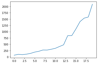
Time_Series

import numpy as np
data_time_series = np.array(data.iloc[:,-1])

import seaborn as sns
from matplotlib import pyplot as plt
ax = sns.lineplot(data = data_time_series)
plt.show()

​

​

加权移动平均 : 蠢

data_time_series_train = data_time_series[0:-2]
data_time_series_test = data_time_series[-2:]

data_time_series_train_array = np.array(data_time_series_train).reshape(1,18)
weight = np.array([0.1,0.2,0.2,0.5])
record = []
for x in range(2,0,-1):
    series = data_time_series_train_array[0,-5-x:-1-x],
    res = np.multiply(series,weight)
    record.append(np.sum(res) + 0.5 * np.sum(res))
    print(" %d : %f" %(2015 - x + 1 , np.sum(res) + 0.5 * np.sum(res)))
    ## res + 0.5res : 加权和 和 提升 蠢
metrics(y_true,record)

 2014 : 1088.397000
 2015 : 1406.899500
mae = 586.26175 , mse = 352723.802464625

Torch : Lstm

补充成任务数据的样式，反归一化输出
我自己怎么可能写得出来呢

# data_time_series : 切出来的 y 一列
data_time_series_lstm = data_time_series
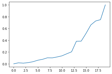
from sklearn.preprocessing import MinMaxScaler
scaler = MinMaxScaler()
max_value = np.max(data_time_series_lstm)
min_value = np.min(data_time_series_lstm)
data_time_series_lstm = (data_time_series_lstm - min_value) / (max_value - min_value)
# std
import seaborn as sns
from matplotlib import pyplot as plt
ax = sns.lineplot(data = data_time_series_lstm)
plt.show()

​

import torch

DAYS_FOR_TRAIN = 5
def create_dataset(data, days_for_train=5) -> (np.array, np.array):
    """
        根据给定的序列data，生成数据集
        数据集分为输入和输出，每一个输入的长度为days_for_train，每一个输出的长度为1。
        也就是说用days_for_train天的数据，对应下一天的数据。
        若给定序列的长度为d，将输出长度为(d-days_for_train+1)个输入/输出对
        数据形式:[x1,x2,x3,x4,y]
    """
    dataset_x, dataset_y= [], []
    for i in range(len(data)-days_for_train):
        _x = data[i:(i+days_for_train)]
        dataset_x.append(_x)
        dataset_y.append(data[i+days_for_train])
    return (np.array(dataset_x), np.array(dataset_y))

dataset_x, dataset_y = create_dataset(data_time_series_lstm, DAYS_FOR_TRAIN)
dataset_y

array([0.06092612, 0.07662843, 0.1023294 , 0.10094056, 0.1164847 ,
       0.13521675, 0.17001685, 0.20355662, 0.38260835, 0.38465949,
       0.51540328, 0.65947204, 0.72668008, 0.74869395, 1.        ])

dataset_y

array([0.06092612, 0.07662843, 0.1023294 , 0.10094056, 0.1164847 ,
       0.13521675, 0.17001685, 0.20355662, 0.38260835, 0.38465949,
       0.51540328, 0.65947204, 0.72668008, 0.74869395, 1.        ])

# 划分训练集和测试集，70%作为训练集
train_size = int(len(dataset_x) * 0.7)

train_x = dataset_x[:train_size]
train_y = dataset_y[:train_size]

# 将数据改变形状，RNN 读入的数据维度是 (seq_size, batch_size, feature_size)
train_x = train_x.reshape(-1, 1, DAYS_FOR_TRAIN)
train_y = train_y.reshape(-1, 1, 1)

# 转为pytorch的tensor对象
train_x = torch.from_numpy(train_x).to(torch.float32)
train_y = torch.from_numpy(train_y).to(torch.float32)

import torch
from torch import nn
class LSTM_Regression(nn.Module):
    """
        使用LSTM进行回归
        参数：
        - input_size: feature size
        - hidden_size: number of hidden units
        - output_size: number of output
        - num_layers: layers of LSTM to stack
    """
    def __init__(self, input_size, hidden_size, output_size=1, num_layers=2):
        super().__init__()
        self.lstm = nn.LSTM(input_size, hidden_size, num_layers)
        self.fc = nn.Linear(hidden_size, output_size)
    def forward(self, _x):
        x, _ = self.lstm(_x)  # _x is input, size (seq_len, batch, input_size)
        s, b, h = x.shape  # x is output, size (seq_len, batch, hidden_size)
        x = x.view(s*b, h)
        x = self.fc(x)
        x = x.view(s, b, -1)  # 把形状改回来
        return x
model = LSTM_Regression(DAYS_FOR_TRAIN, 8, output_size=1, num_layers=2)
loss_function = nn.MSELoss()
optimizer = torch.optim.Adam(model.parameters(), lr=1e-2)

for i in range(100):
    out = model(train_x)
    loss = loss_function(out, train_y)
    loss.backward()
    optimizer.step()
    optimizer.zero_grad()
    if (i+1) % 10 == 0:
        print('Epoch: {}, Loss:{:.5f}'.format(i+1, loss.item()))

Epoch: 10, Loss:0.00674
Epoch: 20, Loss:0.00327
Epoch: 30, Loss:0.00204
Epoch: 40, Loss:0.00116
Epoch: 50, Loss:0.00085
Epoch: 60, Loss:0.00071
Epoch: 70, Loss:0.00064
Epoch: 80, Loss:0.00059
Epoch: 90, Loss:0.00057
Epoch: 100, Loss:0.00055

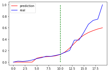
import matplotlib.pyplot as plt
model = model.eval() # 转换成测试模式
# 注意这里用的是全集 模型的输出长度会比原数据少DAYS_FOR_TRAIN 填充使长度相等再作图
dataset_x = dataset_x.reshape(-1, 1, DAYS_FOR_TRAIN)  # (seq_size, batch_size, feature_size)
dataset_x = torch.tensor(dataset_x).to(torch.float32)
pred_test = model(dataset_x) # 全量训练集的模型输出 (seq_size, batch_size, output_size)
pred_test = pred_test.view(-1).data.numpy()
pred_test = np.concatenate((np.zeros(DAYS_FOR_TRAIN), pred_test))  # 填充0 使长度相同
assert len(pred_test) == len(data_time_series_lstm)
plt.plot(pred_test, 'r', label='prediction')
plt.plot(data_time_series_lstm, 'b', label='real')
plt.plot((train_size, train_size), (0, 1), 'g--')
plt.legend(loc='best')
plt.show()

​

​

### 数据反归一化
pred_test =  pred_test * (max_value - pred_test) + pred_test
ax = sns.lineplot(data = pred_test)
plt.show(ax)

​

​

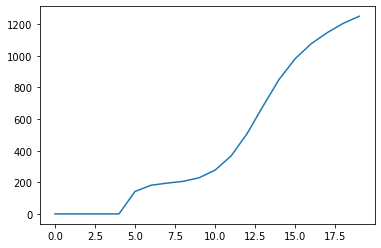
pred_test

array([   0.        ,    0.        ,    0.        ,    0.        ,
          0.        ,  141.97164252,  181.31122203,  194.75042542,
        205.88793585,  228.55081975,  277.00616729,  366.82627218,
        508.25917347,  683.14472015,  851.27406525,  981.55267148,
       1076.44698354, 1146.16705891, 1205.26890924, 1250.06205714])

寄

metrics(data_time_series_lstm, pred_test)

mae = 464.65907024157497 , mse = 414380.31475062034