Model_Bank

import pandas as pd
import numpy as np
from sklearn.model_selection import train_test_split
from sklearn.tree import DecisionTreeClassifier
import seaborn as sns
from sklearn.metrics import confusion_matrix
from matplotlib import pyplot as plt
from sklearn import tree
from sklearn.metrics import accuracy_score
from sklearn.linear_model import LogisticRegression
from sklearn.naive_bayes import GaussianNB
from sklearn.ensemble import RandomForestClassifier, VotingClassifier
from sklearn import svm

# 读取数据
data_load = "work/bankloan.xls"
data = pd.read_excel(data_load)

data.describe()

	年龄	教育	工龄	地址	收入	负债率	信用卡负债	其他负债	违约
count	700.000000	700.000000	700.000000	700.000000	700.000000	700.000000	700.000000	700.000000	700.000000
mean	34.860000	1.722857	8.388571	8.278571	45.601429	10.260571	1.553553	3.058209	0.261429
std	7.997342	0.928206	6.658039	6.824877	36.814226	6.827234	2.117197	3.287555	0.439727
min	20.000000	1.000000	0.000000	0.000000	14.000000	0.400000	0.011696	0.045584	0.000000
25%	29.000000	1.000000	3.000000	3.000000	24.000000	5.000000	0.369059	1.044178	0.000000
50%	34.000000	1.000000	7.000000	7.000000	34.000000	8.600000	0.854869	1.987568	0.000000
75%	40.000000	2.000000	12.000000	12.000000	55.000000	14.125000	1.901955	3.923065	1.000000
max	56.000000	5.000000	31.000000	34.000000	446.000000	41.300000	20.561310	27.033600	1.000000

data.columns

Index(['年龄', '教育', '工龄', '地址', '收入', '负债率', '信用卡负债', '其他负债', '违约'], dtype='object')

data.index

RangeIndex(start=0, stop=700, step=1)

## 转为np 数据切割

X = np.array(data.iloc[:,0:-1])
y = np.array(data.iloc[:,-1])

X_train, X_test, y_train, y_test = train_test_split(X, y, random_state=1, train_size=0.8, test_size=0.2, shuffle=True)

决策树

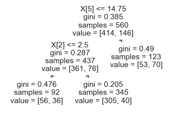
Dtree = DecisionTreeClassifier(max_leaf_nodes=3,random_state=13)
Dtree.fit(X_train, y_train)
y_pred = Dtree.predict(X_test)
accuracy_score(y_test, y_pred)

0.7285714285714285

tree.plot_tree(Dtree)
plt.show()

​

​

## seaborn

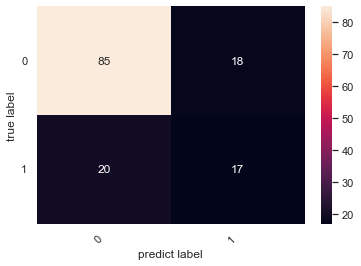
cm = confusion_matrix(y_test, y_pred)
heatmap = sns.heatmap(cm, annot=True, fmt='d')
heatmap.yaxis.set_ticklabels(heatmap.yaxis.get_ticklabels(), rotation=0, ha='right')
heatmap.xaxis.set_ticklabels(heatmap.xaxis.get_ticklabels(), rotation=45, ha='right')
plt.ylabel("true label")
plt.xlabel("predict label")
plt.show()

​

​

SVM

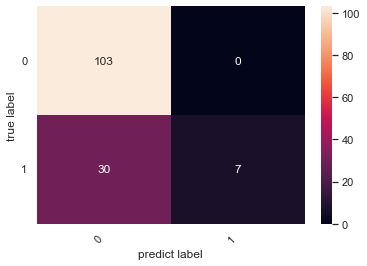
svm = svm.SVC()
svm.fit(X_test,y_test)
y_pred = svm.predict(X_test)
accuracy_score(y_test, y_pred)

0.7857142857142857

cm = confusion_matrix(y_test, y_pred)
heatmap = sns.heatmap(cm, annot=True, fmt='d')
heatmap.yaxis.set_ticklabels(heatmap.yaxis.get_ticklabels(), rotation=0, ha='right')
heatmap.xaxis.set_ticklabels(heatmap.xaxis.get_ticklabels(), rotation=45, ha='right')
plt.ylabel("true label")
plt.xlabel("predict label")
plt.show()

​

​

ensemble

# ensemble
from sklearn import svm
clf1 = LogisticRegression(multi_class='multinomial', random_state=1)
clf2 = RandomForestClassifier(n_estimators=50, random_state=1)
clf3 = GaussianNB()
clf4 = svm.SVC()
clf5 = DecisionTreeClassifier(max_leaf_nodes=3,random_state=13)
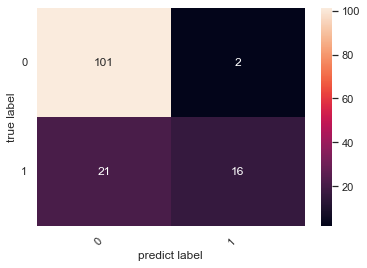
eclf = VotingClassifier(estimators=[
        ('lr', clf1), ('rf', clf2), ('gnb', clf3), ('svm', clf4), ('dtree', clf5)], voting='hard')
eclf = eclf.fit(X, y)
y_pred = eclf.predict(X_test)
accuracy_score(y_test, y_pred)

0.8357142857142857

cm = confusion_matrix(y_test, y_pred)
heatmap = sns.heatmap(cm, annot=True, fmt='d')
heatmap.yaxis.set_ticklabels(heatmap.yaxis.get_ticklabels(), rotation=0, ha='right')
heatmap.xaxis.set_ticklabels(heatmap.xaxis.get_ticklabels(), rotation=45, ha='right')
plt.ylabel("true label")
plt.xlabel("predict label")
plt.show()

​

​

TORCH_BP_NETWORK

import torch
import torch.nn.functional as Fun

train_x = torch.FloatTensor(X_train)
train_y = torch.LongTensor(y_train)
test_x = torch.FloatTensor(X_test)
test_y = torch.LongTensor(y_test)

# BP
class Net(torch.nn.Module):
    def __init__(self, n_feature, n_hidden, n_output):
        super(Net, self).__init__()
        self.hidden = torch.nn.Linear(n_feature, n_hidden)   # 定义隐藏层网络
        self.out = torch.nn.Linear(n_hidden, n_output)   # 定义输出层网络

    def forward(self, x):
        x = Fun.relu(self.hidden(x))      # 隐藏层的激活函数,采用relu,也可以采用sigmod,tanh
        x = self.out(x)                   # 输出层不用激活函数
        return x

net = Net(n_feature=8,n_hidden=20, n_output=2)    #n_feature:输入的特征维度,n_hiddenb:神经元个数,n_output:输出的类别个数
optimizer = torch.optim.SGD(net.parameters(), lr=0.02) # 优化器选用随机梯度下降方式
loss_func = torch.nn.CrossEntropyLoss() # 交叉熵损失函数

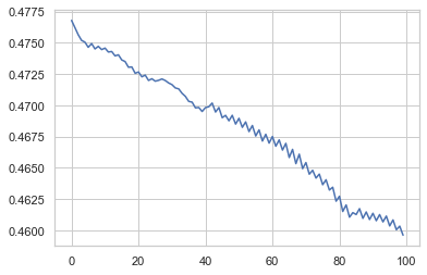
loss_record = []
for t in range(100):
    out = net(train_x)                 # 输入input,输出out
    loss = loss_func(out, train_y)     # 输出与label对比
    loss_record.append(loss.item())
    optimizer.zero_grad()   # 梯度清零
    loss.backward()         # 前馈操作
    optimizer.step()        # 使用梯度优化器

out = net(test_x) #out是一个计算矩阵，可以用Fun.softmax(out)转化为概率矩阵
prediction = torch.max(out, 1)[1] # 返回index  0返回原值
pred_y = prediction.data.numpy()
target_y = test_y.data.numpy()

accuracy = float((pred_y == target_y).astype(int).sum()) / float(target_y.size)
print(accuracy)

0.8071428571428572

##
ax = sns.lineplot(data = loss_record)
plt.show()

​

​

模型读取

torch.save(net, 'work/net.pt')

netC = torch.load('work/net.pt')
input = test_x
output = netC(input)
accuracy = float((pred_y == target_y).astype(int).sum()) / float(target_y.size)
print(accuracy)

0.8071428571428572