
机器学习——森林火灾图片识别
(一)选题背景:森林火灾,是指失去人为控制,在林地内自由蔓延和扩展,对森林、森林生态系统和人类带来一定危害和损失的林火行为。森林火灾是一种突发性强、破坏性大、处置救助较为困难的自然火灾。而近年来由于温室效应加剧,森林火灾频发。在这样的情境下,做好预防是必要的,要做到24小时全天候大范围的监视,卫星、无人机巡查是比较好措施,对于无人机巡查,机器是如何判断当前地区发生火灾,计算机视觉应该是其中一项重要技术,于是设计了对森林火灾图片识别的小程序,希望通过此次的设计对计算机视觉有所理解。
(二)机器学习设计案例设计方案:从网站中下载相关的数据集,对数据集进行整理,在python的环境中,给数据集中的文件打上标签,对数据进行预处理,利用keras,构建网络,训练模型,导入图片测试模型
参考来源:kaggle关于标签学习的讨论区
数据集来源:kaggle,网址:https://www.kaggle.com/
(三)机器学习的实现步骤:
一、二分类
1.下载数据集

2.导入需要用到的库
 1 #导入需要用到的库
 2 import numpy as np
 3 import pandas as pd
 4 import os
 5 import tensorflow as tf
 6 import matplotlib.pyplot as plt
 7 from pathlib import Path
 8 from sklearn.model_selection import train_test_split
 9 from keras.models import Sequential
10 from keras.layers import Activation
11 from keras.layers import Dense, Dropout, Flatten, Conv2D, MaxPooling2D
12 from keras.applications.resnet import preprocess_input
13 from keras_preprocessing.image import ImageDataGenerator
14 from keras.models import load_model
15 from keras.preprocessing.image import load_img, img_to_array
16 from keras import optimizers
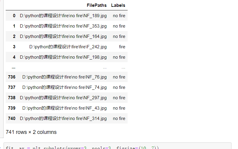
3.遍历数据集中的文件,将路径数据和标签数据生成DataFrame
 1 dir = Path('D:/python的课程设计1/fire')
 2
 3 # 用glob遍历在dir路径中所有jpg格式的文件,并将所有的文件名添加到filepaths列表中
 4 filepaths = list(dir.glob(r'**/*.jpg'))
 5
 6 # 将文件中的分好的小文件名(种类名)分离并添加到labels的列表中
 7 labels = list(map(lambda l: os.path.split(os.path.split(l)[0])[1], filepaths))
 8
 9 # 将filepaths通过pandas转换为Series数据类型
10 filepaths = pd.Series(filepaths, name='FilePaths').astype(str)
11
12 # 将labels通过pandas转换为Series数据类型
13 labels = pd.Series(labels, name='Labels').astype(str)
14
15 # 将filepaths和Series两个Series的数据类型合成DataFrame数据类型
16 df = pd.merge(filepaths, labels, right_index=True, left_index=True)
17 df = df[df['Labels'].apply(lambda l: l[-2:] != 'GT')]
18 df = df.sample(frac=1).reset_index(drop=True)
19 #查看形成的DataFrame的数据
20 df
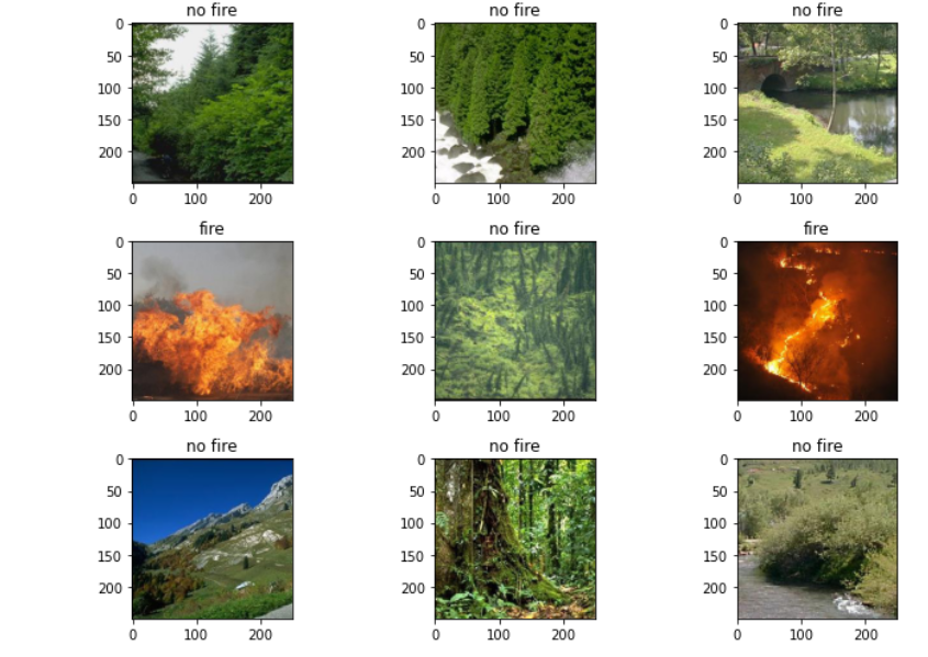
4.查看图像以及对应的标签
 1 #查看图像以及对应的标签
 2 fit, ax = plt.subplots(nrows=3, ncols=3, figsize=(10, 7))
 3
 4 for i, a in enumerate(ax.flat):
 5     a.imshow(plt.imread(df.FilePaths[i]))
 6     a.set_title(df.Labels[i])
 7
 8 plt.tight_layout()
 9 plt.show()
10
11 #查看各个标签的图片张数
12 df['Labels'].value_counts(ascending=True)
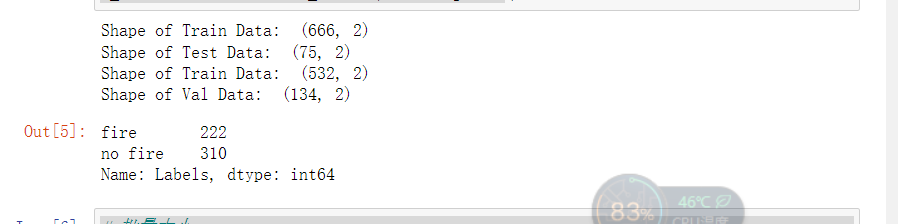
5.由总的数据集生成分别生成训练集,测试集和验证集
 1 #将总数据按10:1的比例分配给X_train, X_test
 2 X_train, X_test = train_test_split(df, test_size=0.1, stratify=df['Labels'])
 3
 4 print('Shape of Train Data: ', X_train.shape)
 5 print('Shape of Test Data: ', X_test.shape)
 6
 7 # 将总数据按5:1的比例分配给X_train, X_train
 8 X_train, X_val = train_test_split(X_train, test_size=0.2, stratify=X_train['Labels'])
 9
10 print('Shape of Train Data: ', X_train.shape)
11 print('Shape of Val Data: ', X_val.shape)
12
13 # 查看各个标签的图片张数
14 X_train['Labels'].value_counts(ascending=True)
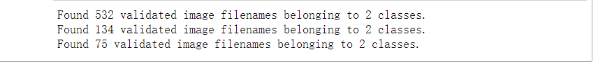
6.图像预处理
 1 # 批量大小
 2 BATCH_SIZE = 32
 3 # 输入图片的大小
 4 IMG_SIZE = (224, 224)
 5
 6 # 图像预处理
 7 img_data_gen = ImageDataGenerator(preprocessing_function=preprocess_input)
 8
 9 X_train = img_data_gen.flow_from_dataframe(dataframe=X_train,
10                                           x_col='FilePaths',
11                                           y_col='Labels',
12                                           target_size=IMG_SIZE,
13                                           color_mode='rgb',
14                                           class_mode='binary',
15                                           batch_size=BATCH_SIZE,
16                                           seed=42)
17
18 X_val = img_data_gen.flow_from_dataframe(dataframe=X_val,
19                                           x_col='FilePaths',
20                                           y_col='Labels',
21                                           target_size=IMG_SIZE,
22                                           color_mode='rgb',
23                                           class_mode='binary',
24                                           batch_size=BATCH_SIZE,
25                                           seed=42)
26 X_test = img_data_gen.flow_from_dataframe(dataframe=X_test,
27                                           x_col='FilePaths',
28                                           y_col='Labels',
29                                           target_size=IMG_SIZE,
30                                           color_mode='rgb',
31                                           class_mode='binary',
32                                           batch_size=BATCH_SIZE,
33                                           seed=42)
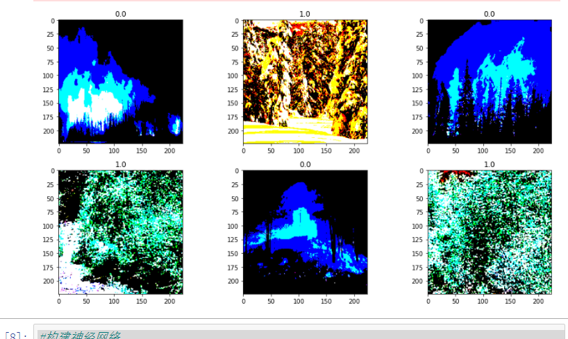
7.查看经过处理的图片以及它的binary标签
#查看经过处理的图片以及它的binary标签
fit, ax = plt.subplots(nrows=2, ncols=3, figsize=(13,7))

for i, a in enumerate(ax.flat):
    img, label = X_train.next()
    a.imshow(img[0],)
    a.set_title(label[0])

plt.tight_layout()
plt.show()
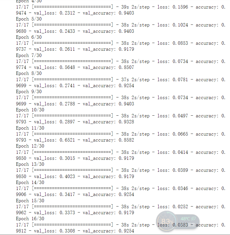
8.构建神经网络并对模型进行训练
#构建神经网络
model = Sequential()
# 数据归一化处理
model.add(tf.keras.layers.experimental.preprocessing.Rescaling(1./255))

# 1.Conv2D层,32个过滤器
model.add(Conv2D(filters=32, kernel_size=(3,3), padding='same', input_shape=(224, 224, 3)))#图形是彩色,‘rgb’,所以设置3
model.add(Activation('relu'))
model.add(MaxPooling2D(pool_size=(2,2), strides=2, padding='valid'))

# 2.Conv2D层,64个过滤器
model.add(Conv2D(filters=64, kernel_size=(3,3), padding='same'))
model.add(Activation('relu'))
model.add(MaxPooling2D(pool_size=(2,2), strides=2, padding='valid'))

# 3.Conv2D层,128个过滤器
model.add(Conv2D(filters=128, kernel_size=(3,3), padding='same'))
model.add(Activation('relu'))
model.add(MaxPooling2D(pool_size=(2,2), strides=2, padding='valid'))

# 将输入层的数据压缩成1维数据,全连接层只能处理一维数据
model.add(Flatten())

# 全连接层
model.add(Dense(256))
model.add(Activation('relu'))

# 减少过拟合
model.add(Dropout(0.5))

# 全连接层
model.add(Dense(1))
model.add(Activation('sigmoid'))

# 模型编译
model.compile(optimizer=optimizers.RMSprop(lr=1e-4),
              loss="categorical_crossentropy",
              metrics=["accuracy"])
#利用批量生成器训练模型
h1 = model.fit(X_train, validation_data=X_val,
epochs=30, )
#保存模型
model.save('t1')
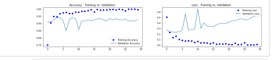
9.绘制损失曲线和精度曲线图
 1 accuracy = h1.history['accuracy']
 2 loss = h1.history['loss']
 3 val_loss = h1.history['val_loss']
 4 val_accuracy = h1.history['val_accuracy']
 5 plt.figure(figsize=(17, 7))
 6 plt.subplot(2, 2, 1)
 7 plt.plot(range(30), accuracy,'bo', label='Training Accuracy')
 8 plt.plot(range(30), val_accuracy, label='Validation Accuracy')
 9 plt.legend(loc='lower right')
10 plt.title('Accuracy : Training vs. Validation ')
11 plt.subplot(2, 2, 2)
12 plt.plot(range(30), loss,'bo' ,label='Training Loss')
13 plt.plot(range(30), val_loss, label='Validation Loss')
14 plt.title('Loss : Training vs. Validation ')
15 plt.legend(loc='upper right')
16 plt.show()
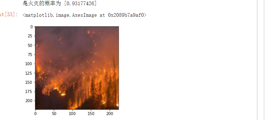
10.导入图片进行预测
from PIL import Image
def con(file,outdir,w=224,h=224):
    img1=Image.open(file)
    img2=img1.resize((w,h),Image.BILINEAR)
    img2.save(os.path.join(outdir,os.path.basename(file)))
file='D:/python的课程设计/NA_Fish_Dataset/Black Sea Sprat/F_23.jpg'
con(file,'D:/python的课程设计/NA_Fish_Dataset/Black Sea Sprat/')
model=load_model('t1')
img_path='D:/python的课程设计/NA_Fish_Dataset/Black Sea Sprat/F_23.jpg'
img = load_img(img_path)
img = img_to_array(img)
img = np.expand_dims(img, axis=0)
out = model.predict(img)
if out[0]>0.5:
        print('是火灾的概率为',out[0])
else:
         print('不是火灾')
img=plt.imread('D:/python的课程设计/NA_Fish_Dataset/Black Sea Sprat/F_23.jpg')
plt.imshow(img)
二、多分类
1.准备数据集

2.遍历数据集中的文件,将路径数据和标签数据生成DataFrame
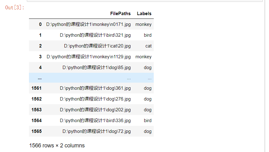
 1 dir = Path('D:/python的课程设计1')
 2
 3 # 用glob遍历在dir路径中所有jpg格式的文件,并将所有的文件名添加到filepaths列表中
 4 filepaths = list(dir.glob(r'**/*.jpg'))
 5
 6 # 将文件中的分好的小文件名(种类名)分离并添加到labels的列表中
 7 labels = list(map(lambda l: os.path.split(os.path.split(l)[0])[1], filepaths))
 8
 9 # 将filepaths通过pandas转换为Series数据类型
10 filepaths = pd.Series(filepaths, name='FilePaths').astype(str)
11
12 # 将labels通过pandas转换为Series数据类型
13 labels = pd.Series(labels, name='Labels').astype(str)
14
15 # 将filepaths和Series两个Series的数据类型合成DataFrame数据类型
16 df = pd.merge(filepaths, labels, right_index=True, left_index=True)
17 df = df[df['Labels'].apply(lambda l: l[-2:] != 'GT')]
18 df = df.sample(frac=1).reset_index(drop=True)
#查看形成的DataFrame的数据
df
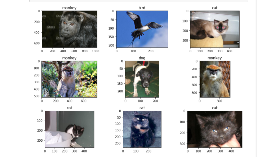
3.查看图像以及对应的标签
1 fit, ax = plt.subplots(nrows=3, ncols=3, figsize=(10, 7))
2
3 for i, a in enumerate(ax.flat):
4     a.imshow(plt.imread(df.FilePaths[i]))
5     a.set_title(df.Labels[i])
6
7 plt.tight_layout()
8 plt.show()
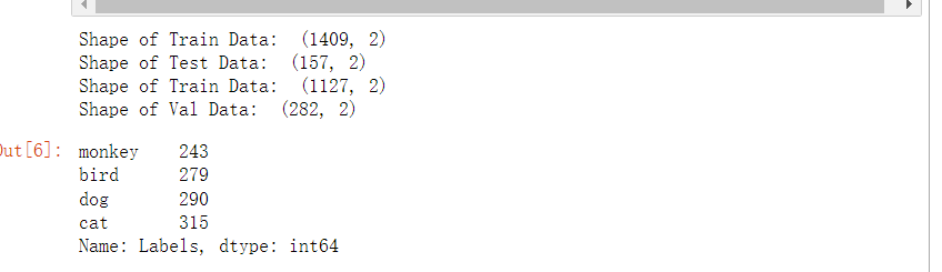
4.由总的数据集生成分别生成训练集,测试集和验证集
#将总数据按10:1的比例分配给X_train, X_test
X_train, X_test = train_test_split(df, test_size=0.1, stratify=df['Labels'])

print('Shape of Train Data: ', X_train.shape)
print('Shape of Test Data: ', X_test.shape)

# 将总数据按5:1的比例分配给X_train, X_train
X_train, X_val = train_test_split(X_train, test_size=0.2, stratify=X_train['Labels'])

print('Shape of Train Data: ', X_train.shape)
print('Shape of Val Data: ', X_val.shape)

# 查看各个标签的图片张数
X_train['Labels'].value_counts(ascending=True)
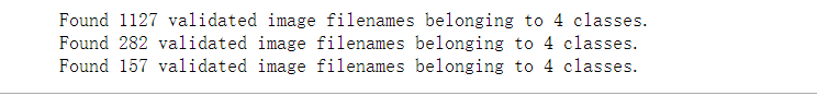
5.图像预处理
 1 # 批量的大小
 2 BATCH_SIZE = 32
 3 # 输入图片的大小
 4 IMG_SIZE = (224, 224)
 5
 6 # 图像预处理
 7 img_data_gen = ImageDataGenerator(preprocessing_function=preprocess_input)
 8
 9
10 X_train = img_data_gen.flow_from_dataframe(dataframe=X_train,
11                                           x_col='FilePaths',
12                                           y_col='Labels',
13                                           target_size=IMG_SIZE,
14                                           color_mode='rgb',
15                                           class_mode='categorical',
16                                           batch_size=BATCH_SIZE,
17                                           seed=42)
18
19 X_val = img_data_gen.flow_from_dataframe(dataframe=X_val,
20                                           x_col='FilePaths',
21                                           y_col='Labels',
22                                           target_size=IMG_SIZE,
23                                           color_mode='rgb',
24                                           class_mode='categorical',
25                                           batch_size=BATCH_SIZE,
26                                           seed=42)
27 X_test = img_data_gen.flow_from_dataframe(dataframe=X_test,
28                                           x_col='FilePaths',
29                                           y_col='Labels',
30                                           target_size=IMG_SIZE,
31                                           color_mode='rgb',
32                                           class_mode='categorical',
33                                           batch_size=BATCH_SIZE,
34                                           seed=42)
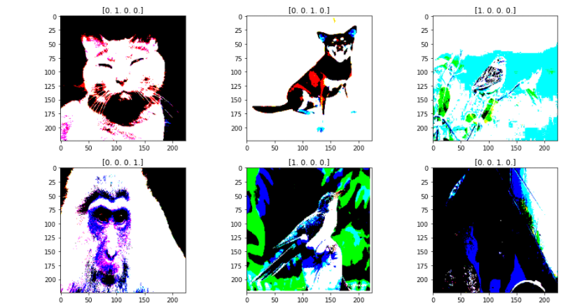
6.查看经过处理的图片以及它的one-hot标签
1 fit, ax = plt.subplots(nrows=2, ncols=3, figsize=(13,7))
2
3 for i, a in enumerate(ax.flat):
4     img, label = X_train.next()
5     a.imshow(img[0],)
6     a.set_title(label[0])
7
8 plt.tight_layout()
9 plt.show()
7.构建神经网络并训练模型
 1 model = Sequential()
 2 # 数据归一化处理
 3 model.add(tf.keras.layers.experimental.preprocessing.Rescaling(1./255))
 4
 5 # 1.Conv2D层,32个过滤器
 6 model.add(Conv2D(filters=32, kernel_size=(3,3), padding='same', input_shape=(224, 224, 3)))#图形是彩色,‘rgb’,所以设置3
 7 model.add(Activation('relu'))
 8 model.add(MaxPooling2D(pool_size=(2,2), strides=2, padding='valid'))
 9
10 # 2.Conv2D层,64个过滤器
11 model.add(Conv2D(filters=64, kernel_size=(3,3), padding='same'))
12 model.add(Activation('relu'))
13 model.add(MaxPooling2D(pool_size=(2,2), strides=2, padding='valid'))
14
15 # 3.Conv2D层,128个过滤器
16 model.add(Conv2D(filters=128, kernel_size=(3,3), padding='same'))
17 model.add(Activation('relu'))
18 model.add(MaxPooling2D(pool_size=(2,2), strides=2, padding='valid'))
19
20 # 将输入层的数据压缩成1维数据,全连接层只能处理一维数据
21 model.add(Flatten())
22
23 # 全连接层
24 model.add(Dense(256))
25 model.add(Activation('relu'))
26
27 # 减少过拟合
28 model.add(Dropout(0.5))
29
30 # 全连接层
31 model.add(Dense(4))#需要识别的有4个种类
32 model.add(Activation('softmax'))#softmax是基于二分类函数sigmoid的多分类函数
33
34 # 模型编译
35 model.compile(optimizer=optimizers.RMSprop(lr=1e-4),
36               loss="categorical_crossentropy",
37               metrics=["accuracy"])
38 #利用批量生成器训练模型
39 h1 = model.fit(X_train, validation_data=X_val,
40                epochs=30, )
41 #保存模型
42 model.save('h21')
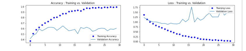
8.绘制损失曲线和精度曲线图
 1 accuracy = h1.history['accuracy']
 2 loss = h1.history['loss']
 3 val_loss = h1.history['val_loss']
 4 val_accuracy = h1.history['val_accuracy']
 5 plt.figure(figsize=(17, 7))
 6 plt.subplot(2, 2, 1)
 7 plt.plot(range(30), accuracy,'bo', label='Training Accuracy')
 8 plt.plot(range(30), val_accuracy, label='Validation Accuracy')
 9 plt.legend(loc='lower right')
10 plt.title('Accuracy : Training vs. Validation ')
11 plt.subplot(2, 2, 2)
12 plt.plot(range(30), loss,'bo' ,label='Training Loss')
13 plt.plot(range(30), val_loss, label='Validation Loss')
14 plt.title('Loss : Training vs. Validation ')
15 plt.legend(loc='upper right')
16 plt.show()
9.用ImageDataGenerator数据增强
train_datagen = ImageDataGenerator(rescale=1./255,
                                  rotation_range=40, #将图像随机旋转40度
                                  width_shift_range=0.2, #在水平方向上平移比例为0.2
                                  height_shift_range=0.2, #在垂直方向上平移比例为0.2
                                  shear_range=0.2, #随机错切变换的角度为0.2
                                  zoom_range=0.2, #图片随机缩放的范围为0.2
                                  horizontal_flip=True, #随机将一半图像水平翻转
                                  fill_mode='nearest') #填充创建像素

X_val1 = ImageDataGenerator(rescale=1./255)

X_train1 = train_datagen.flow_from_dataframe(
                        X_train,
                        target_size=(150,150),
                        batch_size=32,
                        class_mode='categorical'
                        )

X_val1= test_datagen.flow_from_dataframe(
                        X_test,
                        target_size=(150,150),
                        batch_size=32,
                        class_mode='categorical')
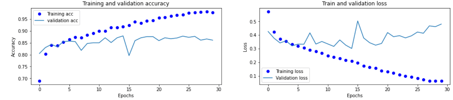
再次训练模型,并绘制绘制损失曲线和精度曲线图,得到结果图
10.导入图片进行预测
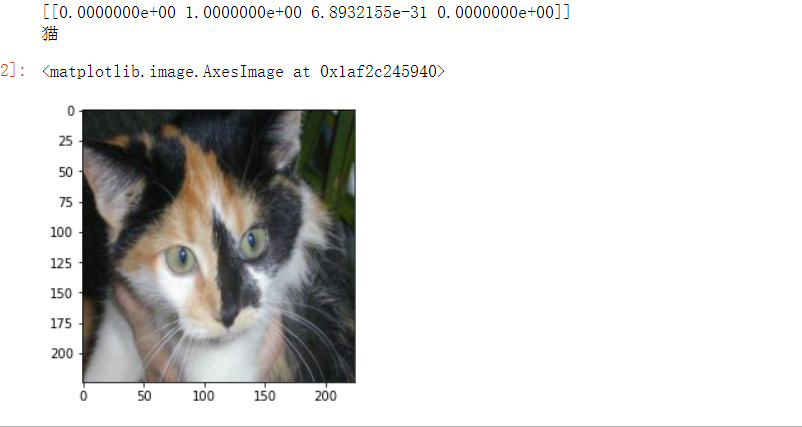
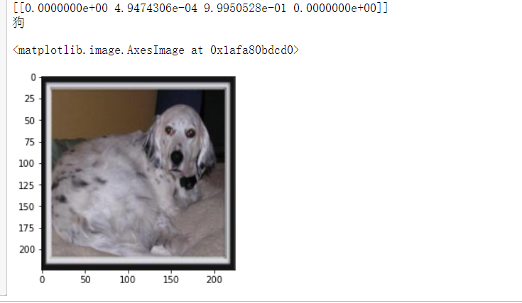
 1 from PIL import Image
 2 def con(file,outdir,w=224,h=224):
 3     img1=Image.open(file)
 4     img2=img1.resize((w,h),Image.BILINEAR)
 5     img2.save(os.path.join(outdir,os.path.basename(file)))
 6 file='D:/python的课程设计/预测/414.jpg'
 7 con(file,'D:/python的课程设计/预测/')
 8 model=load_model('h20')
 9 img_path='D:/python的课程设计/预测/414.jpg'
10 img = load_img(img_path)
11 img = img_to_array(img)
12 img = np.expand_dims(img, axis=0)
13 out = model.predict(img)
14 print(out)
15 dict={'0':'鸟','1':'猫','2':'狗','3':'猴子'}
16 for i in range(4):
17     if out[0][i]>0.5:
18         print(dict[str(i)])
19 img=plt.imread('D:/python的课程设计/预测/414.jpg')
20 plt.imshow(img)
 1 file='D:/python的课程设计/预测/512.jpg'
 2 con(file,'D:/python的课程设计/预测/')
 3 model=load_model('h20')
 4 img_path='D:/python的课程设计/预测/512.jpg'
 5 img = load_img(img_path)
 6 img = img_to_array(img)
 7 img = np.expand_dims(img, axis=0)
 8 out = model.predict(img)
 9 print(out)
10 dict={'0':'鸟','1':'猫','2':'狗','3':'猴子'}
11 for i in range(4):
12     if out[0][i]>0.5:
13         print(dict[str(i)])
14 img=plt.imread('D:/python的课程设计/预测/512.jpg')
15 plt.imshow(img)
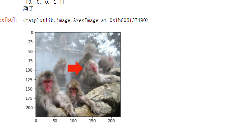
 1 file='D:/python的课程设计/预测/n3044.jpg'
 2 con(file,'D:/python的课程设计/预测/')
 3 model=load_model('h20')
 4 img_path='D:/python的课程设计/预测/n3044.jpg'
 5 img = load_img(img_path)
 6 img = img_to_array(img)
 7 img = np.expand_dims(img, axis=0)
 8 out = model.predict(img)
 9 print(out)
10 dict={'0':'鸟','1':'猫','2':'狗','3':'猴子'}
11 for i in range(4):
12     if out[0][i]>0.5:
13         print(dict[str(i)])
14 img=plt.imread('D:/python的课程设计/预测/n3044.jpg')
15 plt.imshow(img)
全部代码附上:
  1 #导入需要用到的库
  2 import numpy as np
  3 import pandas as pd
  4 import os
  5 import tensorflow as tf
  6 import matplotlib.pyplot as plt
  7 from pathlib import Path
  8 from sklearn.model_selection import train_test_split
  9 from keras.models import Sequential
 10 from keras.layers import Activation
 11 from keras.layers import Dense, Dropout, Flatten, Conv2D, MaxPooling2D
 12 from keras.applications.resnet import preprocess_input
 13 from keras_preprocessing.image import ImageDataGenerator
 14 from keras.models import load_model
 15 from keras.preprocessing.image import load_img, img_to_array
 16 from keras import optimizers
 17
 18 dir = Path('D:/python的课程设计/fire')
 19
 20 # 用glob遍历在dir路径中所有jpg格式的文件,并将所有的文件名添加到filepaths列表中
 21 filepaths = list(dir.glob(r'**/*.jpg'))
 22
 23 # 将文件中的分好的小文件名(种类名)分离并添加到labels的列表中
 24 labels = list(map(lambda l: os.path.split(os.path.split(l)[0])[1], filepaths))
 25
 26 # 将filepaths通过pandas转换为Series数据类型
 27 filepaths = pd.Series(filepaths, name='FilePaths').astype(str)
 28
 29 # 将labels通过pandas转换为Series数据类型
 30 labels = pd.Series(labels, name='Labels').astype(str)
 31
 32 # 将filepaths和Series两个Series的数据类型合成DataFrame数据类型
 33 df = pd.merge(filepaths, labels, right_index=True, left_index=True)
 34 df = df[df['Labels'].apply(lambda l: l[-2:] != 'GT')]
 35 df = df.sample(frac=1).reset_index(drop=True)
 36 #查看形成的DataFrame的数据
 37 df
 38 #查看图像以及对应的标签
 39 fit, ax = plt.subplots(nrows=3, ncols=3, figsize=(10, 7))
 40
 41 for i, a in enumerate(ax.flat):
 42     a.imshow(plt.imread(df.FilePaths[i]))
 43     a.set_title(df.Labels[i])
 44
 45 plt.tight_layout()
 46 plt.show()
 47
 48 # 由总的数据集生成分别生成训练集,测试集和验证集
 49 #将总数据按10:1的比例分配给X_train, X_test
 50 X_train, X_test = train_test_split(df, test_size=0.1, stratify=df['Labels'])
 51
 52 print('Shape of Train Data: ', X_train.shape)
 53 print('Shape of Test Data: ', X_test.shape)
 54
 55 # 将总数据按5:1的比例分配给X_train, X_train
 56 X_train, X_val = train_test_split(X_train, test_size=0.2, stratify=X_train['Labels'])
 57
 58 print('Shape of Train Data: ', X_train.shape)
 59 print('Shape of Val Data: ', X_val.shape)
 60
 61 # 查看各个标签的图片张数
 62 X_train['Labels'].value_counts(ascending=True)
 63
 64 # 批量大小
 65 BATCH_SIZE = 32
 66 # 输入图片的大小
 67 IMG_SIZE = (224, 224)
 68
 69 # 图像预处理
 70 img_data_gen = ImageDataGenerator(preprocessing_function=preprocess_input)
 71
 72 X_train = img_data_gen.flow_from_dataframe(dataframe=X_train,
 73                                           x_col='FilePaths',
 74                                           y_col='Labels',
 75                                           target_size=IMG_SIZE,
 76                                           color_mode='rgb',
 77                                           class_mode='binary',
 78                                           batch_size=BATCH_SIZE,
 79                                           seed=42)
 80
 81 X_val = img_data_gen.flow_from_dataframe(dataframe=X_val,
 82                                           x_col='FilePaths',
 83                                           y_col='Labels',
 84                                           target_size=IMG_SIZE,
 85                                           color_mode='rgb',
 86                                           class_mode='binary',
 87                                           batch_size=BATCH_SIZE,
 88                                           seed=42)
 89 X_test = img_data_gen.flow_from_dataframe(dataframe=X_test,
 90                                           x_col='FilePaths',
 91                                           y_col='Labels',
 92                                           target_size=IMG_SIZE,
 93                                           color_mode='rgb',
 94                                           class_mode='binary',
 95                                           batch_size=BATCH_SIZE,
 96                                           seed=42)
 97
 98 #查看经过处理的图片以及它的binary标签
 99 fit, ax = plt.subplots(nrows=2, ncols=3, figsize=(13,7))
100
101 for i, a in enumerate(ax.flat):
102     img, label = X_train.next()
103     a.imshow(img[0],)
104     a.set_title(label[0])
105
106 plt.tight_layout()
107 plt.show()
108
109 #构建神经网络
110 model = Sequential()
111 # 数据归一化处理
112 model.add(tf.keras.layers.experimental.preprocessing.Rescaling(1./255))
113
114 # 1.Conv2D层,32个过滤器
115 model.add(Conv2D(filters=32, kernel_size=(3,3), padding='same', input_shape=(224, 224, 3)))#图形是彩色,‘rgb’,所以设置3
116 model.add(Activation('relu'))
117 model.add(MaxPooling2D(pool_size=(2,2), strides=2, padding='valid'))
118
119 # 2.Conv2D层,64个过滤器
120 model.add(Conv2D(filters=64, kernel_size=(3,3), padding='same'))
121 model.add(Activation('relu'))
122 model.add(MaxPooling2D(pool_size=(2,2), strides=2, padding='valid'))
123
124 # 3.Conv2D层,128个过滤器
125 model.add(Conv2D(filters=128, kernel_size=(3,3), padding='same'))
126 model.add(Activation('relu'))
127 model.add(MaxPooling2D(pool_size=(2,2), strides=2, padding='valid'))
128
129 # 将输入层的数据压缩成1维数据,全连接层只能处理一维数据
130 model.add(Flatten())
131
132 # 全连接层
133 model.add(Dense(256))
134 model.add(Activation('relu'))
135
136 # 减少过拟合
137 model.add(Dropout(0.5))
138
139 # 全连接层
140 model.add(Dense(1))
141 model.add(Activation('sigmoid'))
142
143 # 模型编译
144 model.compile(optimizer=optimizers.RMSprop(lr=1e-4),
145               loss="categorical_crossentropy",
146               metrics=["accuracy"])
147 #利用批量生成器训练模型
148 h1 = model.fit(X_train, validation_data=X_val,
149                epochs=30, )
150 #保存模型
151 model.save('t1')
152
153 #绘制损失曲线和精度曲线图
154 accuracy = h1.history['accuracy']
155 loss = h1.history['loss']
156 val_loss = h1.history['val_loss']
157 val_accuracy = h1.history['val_accuracy']
158 plt.figure(figsize=(17, 7))
159 plt.subplot(2, 2, 1)
160 plt.plot(range(30), accuracy,'bo', label='Training Accuracy')
161 plt.plot(range(30), val_accuracy, label='Validation Accuracy')
162 plt.legend(loc='lower right')
163 plt.title('Accuracy : Training vs. Validation ')
164 plt.subplot(2, 2, 2)
165 plt.plot(range(30), loss,'bo' ,label='Training Loss')
166 plt.plot(range(30), val_loss, label='Validation Loss')
167 plt.title('Loss : Training vs. Validation ')
168 plt.legend(loc='upper right')
169 plt.show()
170
171 from PIL import Image
172 def con(file,outdir,w=224,h=224):
173     img1=Image.open(file)
174     img2=img1.resize((w,h),Image.BILINEAR)
175     img2.save(os.path.join(outdir,os.path.basename(file)))
176 file='D:/python的课程设计/NA_Fish_Dataset/Black Sea Sprat/F_23.jpg'
177 con(file,'D:/python的课程设计/NA_Fish_Dataset/Black Sea Sprat/')
178 model=load_model('t1')
179 img_path='D:/python的课程设计/NA_Fish_Dataset/Black Sea Sprat/F_23.jpg'
180 img = load_img(img_path)
181 img = img_to_array(img)
182 img = np.expand_dims(img, axis=0)
183 out = model.predict(img)
184 if out[0]>0.5:
185         print('是火灾的概率为',out[0])
186 else:
187          print('不是火灾')
188 img=plt.imread('D:/python的课程设计/NA_Fish_Dataset/Black Sea Sprat/F_23.jpg')
189 plt.imshow(img)
190
191 dir = Path('D:/python的课程设计1')
192
193 # 用glob遍历在dir路径中所有jpg格式的文件,并将所有的文件名添加到filepaths列表中
194 filepaths = list(dir.glob(r'**/*.jpg'))
195
196 # 将文件中的分好的小文件名(种类名)分离并添加到labels的列表中
197 labels = list(map(lambda l: os.path.split(os.path.split(l)[0])[1], filepaths))
198
199 # 将filepaths通过pandas转换为Series数据类型
200 filepaths = pd.Series(filepaths, name='FilePaths').astype(str)
201
202 # 将labels通过pandas转换为Series数据类型
203 labels = pd.Series(labels, name='Labels').astype(str)
204
205 # 将filepaths和Series两个Series的数据类型合成DataFrame数据类型
206 df = pd.merge(filepaths, labels, right_index=True, left_index=True)
207 df = df[df['Labels'].apply(lambda l: l[-2:] != 'GT')]
208 df = df.sample(frac=1).reset_index(drop=True)
209
210 #构建神经网络
211 model = Sequential()
212 # 数据归一化处理
213 model.add(tf.keras.layers.experimental.preprocessing.Rescaling(1./255))
214
215 # 1.Conv2D层,32个过滤器
216 model.add(Conv2D(filters=32, kernel_size=(3,3), padding='same', input_shape=(224, 224, 3)))#图形是彩色,‘rgb’,所以设置3
217 model.add(Activation('relu'))
218 model.add(MaxPooling2D(pool_size=(2,2), strides=2, padding='valid'))
219
220 # 2.Conv2D层,64个过滤器
221 model.add(Conv2D(filters=64, kernel_size=(3,3), padding='same'))
222 model.add(Activation('relu'))
223 model.add(MaxPooling2D(pool_size=(2,2), strides=2, padding='valid'))
224
225 # 3.Conv2D层,128个过滤器
226 model.add(Conv2D(filters=128, kernel_size=(3,3), padding='same'))
227 model.add(Activation('relu'))
228 model.add(MaxPooling2D(pool_size=(2,2), strides=2, padding='valid'))
229
230 # 将输入层的数据压缩成1维数据,全连接层只能处理一维数据
231 model.add(Flatten())
232
233 # 全连接层
234 model.add(Dense(256))
235 model.add(Activation('relu'))
236
237 # 减少过拟合
238 model.add(Dropout(0.5))
239
240 # 全连接层
241 model.add(Dense(4))#需要识别的有4个种类
242 model.add(Activation('softmax'))#softmax是基于二分类函数sigmoid的多分类函数
243
244 # 模型编译
245 model.compile(optimizer=optimizers.RMSprop(lr=1e-4),
246               loss="categorical_crossentropy",
247               metrics=["accuracy"])
248 #利用批量生成器训练模型
249 h1 = model.fit(X_train, validation_data=X_val,
250                epochs=30, )
251 #保存模型
252 model.save('h21')
253
254
255 #绘制损失曲线和精度曲线图
256 accuracy = h1.history['accuracy']
257 loss = h1.history['loss']
258 val_loss = h1.history['val_loss']
259 val_accuracy = h1.history['val_accuracy']
260 plt.figure(figsize=(17, 7))
261 plt.subplot(2, 2, 1)
262 plt.plot(range(30), accuracy,'bo', label='Training Accuracy')
263 plt.plot(range(30), val_accuracy, label='Validation Accuracy')
264 plt.legend(loc='lower right')
265 plt.title('Accuracy : Training vs. Validation ')
266 plt.subplot(2, 2, 2)
267 plt.plot(range(30), loss,'bo' ,label='Training Loss')
268 plt.plot(range(30), val_loss, label='Validation Loss')
269 plt.title('Loss : Training vs. Validation ')
270 plt.legend(loc='upper right')
271 plt.show()
272
273 #定义ImageDataGenerator参数
274 train_datagen = ImageDataGenerator(rescale=1./255,
275                                   rotation_range=40, #将图像随机旋转40度
276                                   width_shift_range=0.2, #在水平方向上平移比例为0.2
277                                   height_shift_range=0.2, #在垂直方向上平移比例为0.2
278                                   shear_range=0.2, #随机错切变换的角度为0.2
279                                   zoom_range=0.2, #图片随机缩放的范围为0.2
280                                   horizontal_flip=True, #随机将一半图像水平翻转
281                                   fill_mode='nearest') #填充创建像素
282
283 X_val1 = ImageDataGenerator(rescale=1./255)
284
285 X_train1 = train_datagen.flow_from_dataframe(
286                         X_train,
287                         target_size=(150,150),
288                         batch_size=32,
289                         class_mode='categorical'
290                         )
291
292 X_val1= test_datagen.flow_from_dataframe(
293                         X_test,
294                         target_size=(150,150),
295                         batch_size=32,
296                         class_mode='categorical')
297
298 from PIL import Image
299 def con(file,outdir,w=224,h=224):
300     img1=Image.open(file)
301     img2=img1.resize((w,h),Image.BILINEAR)
302     img2.save(os.path.join(outdir,os.path.basename(file)))
303 file='D:/python的课程设计/预测/414.jpg'
304 con(file,'D:/python的课程设计/预测/')
305 model=load_model('h21')
306 img_path='D:/python的课程设计/预测/414.jpg'
307 img = load_img(img_path)
308 img = img_to_array(img)
309 img = np.expand_dims(img, axis=0)
310 out = model.predict(img)
311 print(out)
312 dict={'0':'鸟','1':'猫','2':'狗','3':'猴子'}
313 for i in range(4):
314     if out[0][i]>0.5:
315         print(dict[str(i)])
316 img=plt.imread('D:/python的课程设计/预测/414.jpg')
317 plt.imshow(img)
(四)总结:本次的程序设计主要内容是机器学习的标签学习,通过本次课程设计,加深了我对机器学习以及其标签学习的理解。
机器学习就是通过利用数据,训练模型,然后模型预测的一种方法。这次学习主要是对二分类和多分类进行实践。二分类:所用到的二分类函数即sigmoid,而多分类用到的则是softmax基于二分类的多分类函数。sigmoid是对每一个输出值进行非线性化,而sofmax则是计算比重,二者结果相似,都具有归一作用,但softmax是一个针对输出结果归一化的过程sigmoid是则是一个非线性激活过程,即当输出层为一个神经元时会用sigmoid,softmax一般和one-hot标签配合使用,一般用于网络的最后一层,sigmoid与0,1真实标签配合使用。使用softmax时应将损失函数设置为categorical_crossentropy损失函数,而使用sigmoid时则将损失函数设置为binary_crossentropy损失函数。
本次程序设计的不足:在数据增强上效果不是很明显,在设计过程中还遇到图像失真导致训练精度上升缓慢

 浙公网安备 33010602011771号