【机器学习实战】分类

获取数据集MNIST

# mnist: handwritten numbers represented by pixels

# get the dataset
from sklearn.datasets import fetch_openml
mnist = fetch_openml("mnist_784", version=1)

print(mnist.keys())
# dict_keys(['data', 'target', 'frame', 'categories', 'feature_names', 'target_names', 'DESCR', 'details', 'url'])

X, y = mnist['data'], mnist['target']

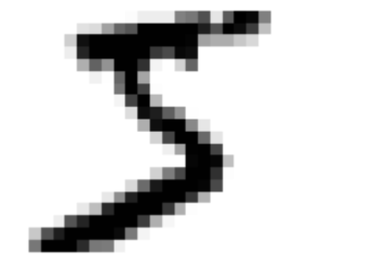
# an example to explore the data
import matplotlib as mpl
import matplotlib.pyplot as plt

some_digit = X[0:1]
some_digit = some_digit.values                 # transform DataFrame to Array
some_digit_image = some_digit.reshape(28, 28)  # 1*784 -> 28*28  (rows*colums)

plt.imshow(some_digit_image, cmap= 'binary')
plt.axis('off')
plt.show()

# transform y to numbers
import numpy as np
y = y.astype(np.uint8)

训练二元分类模型

# data processing
X_train, X_test, y_train, y_test = X[:60000], X[60000:], y[:60000], y[60000:]
y_train_5 = (y_train == 5)
y_test_5 = (y_test == 5)

# Stochastic Gradient Descent (SGD)
from sklearn.linear_model import SGDClassifier

sgd_clf = SGDClassifier(random_state=42)
sgd_clf.fit(X_train, y_train_5)

# predict
sgd_clf.predict(some_digit)
# out: array([ True])

性能测量

k折交叉验证

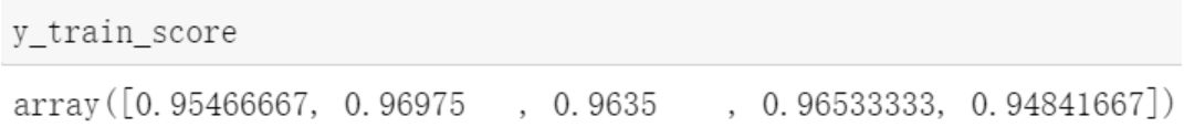
from sklearn.model_selection import cross_val_score

y_train_score = cross_val_score(sgd_clf, X_train, y_train_5, scoring='accuracy')  # default cv=5

from sklearn.base import BaseEstimator

class Never5Classifier(BaseEstimator):
    def fit(self, X, y=None):
        return self
    def predict(self, X):
        return np.zeros((len(X),1), dtype=bool)
    
never_5_clf = Never5Classifier()
never_5_score = cross_val_score(never_5_clf, X_train, y_train_5, scoring='accuracy')

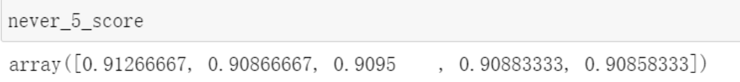
分析：当处理有偏数据集（某些类比其他类更为频繁），准确率往往无法成为分类器的首要性能指标

# cross_val_predict ：k-fold cross validation as well
# output the  clean predicted result 
# ('clean' means the predicted data hasn't seen when training)
from sklearn.model_selection import cross_val_predict
y_pred = cross_val_predict(sgd_clf, X_train, y_train_5, cv=3)

# confusion matrix
from sklearn.metrics import confusion_matrix
confusion_matrix(y_train_5, y_pred)

y_perfect_pred = y_train_5
confusion_matrix(y_train_5, y_perfect_pred)

confusion matrix (2 elems as example):
                      Predicted
Actual       array ( [ [ TN,     FP],
                       [ FN,     TP] ] )
           
TN 真负类  FP 假正类  FN 假正类  TP 真正类

精度和召回率

精度：    TP / ( TP + FP)
召回率：  TP / ( TP + FN)
F1分数：  精度和召回率的调和平均

from sklearn.metrics import precision_score, recall_score, f1_score
precision_score(y_train_5, y_pred)
# 0.8370879772350012

recall_score(y_train_5, y_pred)
# 0.6511713705958311

f1_score(y_train_5, y_pred)
# 0.7325171197343846

精度和召回率不可兼得，例如：
给儿童过滤合适的网站，要求精度高；
监控小偷偷盗，要求召回率高

精度/召回率平衡

SGDClassifier根据决策函数计算分值，若大于阈值，将该实例判为正类；否则判为负类
阈值越高，精度越高，召回率越低；阈值越低，精度越低，召回率越高

Scikit-Learn不允许直接设置阈值，但可以访问它用于预测的决策分数
调用decision_function()方法，返回每个实例的分数。根据这些分数，对任意阈值进行预测：

y_scores = sgd_clf.decision_function(some_digit)
>>> y_scores
>>> array([2164.22030239])

threshold = 0
y_some_digit_pred = (y_scores > threshold)
>>> y_some_digit_pred
>>> array([ True])

from sklearn.model_selection import cross_val_score, cross_val_predict

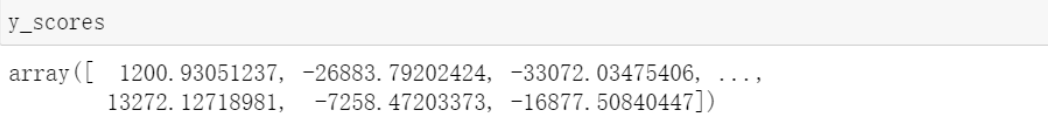
# get the scores of the training data
y_scores = cross_val_predict(sgd_clf, X_train, y_train_5, cv=3, method='decision_function')

from sklearn.metrics import precision_recall_curve

precisions, recalls, thresholds = precision_recall_curve(y_train_5, y_scores)

def plot_precision_recall_vs_threshold(precisions, recalls, threshold):
    plt.plot(thresholds, precisions[:-1], 'b--', label='Precision')
    plt.plot(thresholds, recalls[:-1], 'g-', label='Recall')
    
plot_precision_recall_vs_threshold(precisions, recalls, thresholds)
plt.show()

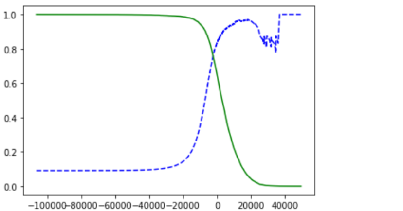
注：提高阈值时，精度可能下降。所以精度曲线要更崎岖一些。

from sklearn.metrics import precision_score, recall_score

threshold_90_precision = thresholds[np.argmax(precisions >= 0.90)]  # np.argmax()返回第一个True的索引
y_train_pred_90 = (y_scores >= threshold_90_precision)

>>> precision_score(y_train_5, y_train_pred_90)
>>> 0.9000345901072293
>>> recall_score(y_train_5, y_train_pred_90)
>>> 0.4799852425751706

ROC曲线

假正率–真正率（召回率）

from sklearn.model_selection import cross_val_predict

y_scores = cross_val_predict(sgd_clf, X_train, y_train_5, cv=3, method='decision_function')

from sklearn.metrics import roc_curve

fpr, tpr, thresholds = roc_curve(y_train_5, y_scores)

def plot_roc_curve(fpr, tpr, label=None):
    plt.plot(fpr, tpr, linewidth=2, label=label)
    plt.plot([0, 1], [0, 1], 'k--')
    
plot_roc_curve(fpr, tpr)
plt.show()

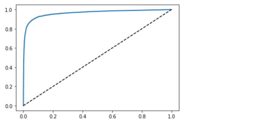
召回率（TPR）越高，分类器产生的假正类（FPR）越多
虚线表示纯随机分类器的ROC曲线，优秀的分类器应该越远离这条线越好（左上角）

一种比较分类器的方法是测量曲线下面积（AUC），完美的分类器ROC AUC等于1，纯随机分类器为0.5

from sklearn.metrics import roc_auc_score
roc_auc_score(y_train_5, y_scores)
#out:0.964343966522447

多类分类器

一对剩余（OvR) / 一对多（one-versus-all) 策略：
若创建一个系统将样本分为N类，训练N个分类器，每个类一个——1-检测器，2-检测器……N-检测器（这里类的标签用数字编号表示）
当对一个样本进行预测时，获取每个分类器的决策分数，将其分到对应分类器最高的类
一对一（OvO）策略：
对每一对类训练一个分类器——区分1-2， 1-3， 2-3……
如果存在N个类，则需训练N*（N-1）/2个分类器，其优点在于每个分类器只需用到部分训练集对其必须区分的两个类进行训练

以下例子数据的获取与初步处理同前

from sklearn.svm import SVC

svm_clf = SVC()
svm_clf.fit(X_train, y_train)

svm_clf.predict(some_digit)
#output: 5

some_digit_scores = svm_clf.decision_function(some_digit)

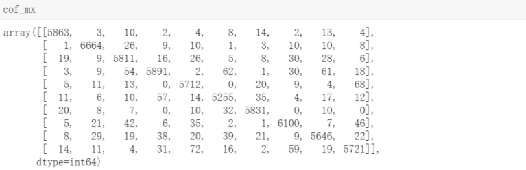
from sklearn.metrics import confusion_matrix
from sklearn.model_selection import cross_val_predict

y_pred = cross_val_predict(svm_clf, X_train, y_train, cv=3)
cof_mx = confusion_matrix(y_train, y_pred)

import matplotlib as mpl
import matplotlib.pyplot as plt

plt.matshow(cof_mx, cmap=plt.cm.gray)
plt.show()

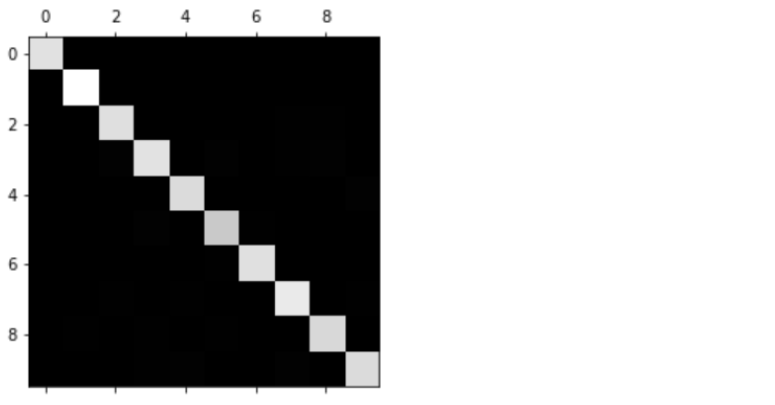
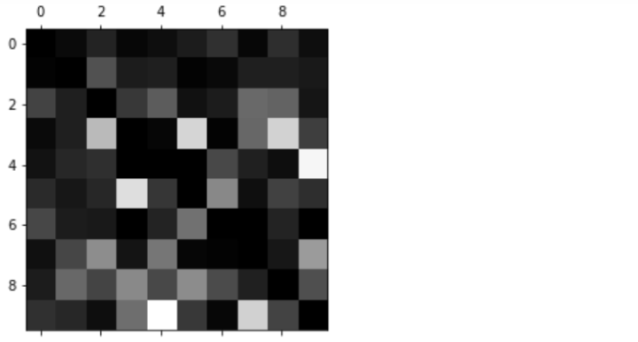
为关注分类错误情况：

row_sums = cof_mx.sum(axis=1, keepdims = True)
cof_mx = cof_mx / row_sums

import numpy as np
np.fill_diagonal(cof_mx, 0)

plt.matshow(cof_mx, cmap=plt.cm.gray)
plt.show()

多标签分类

输入一个样本，可以输出多个类

from sklearn.neighbors import KNeighborsClassifier

y_train_large = (y_train >= 7)
y_train_odd = (y_train % 2 == 1)
y_multilabel = np.c_[y_train_large, y_train_odd]

knn_clf = KNeighborsClassifier()
knn_clf.fit(X_train, y_multilabel)

from sklearn.metrics import f1_score
y_train_knn_pred = cross_val_predict(knn_clf, X_train, y_multilabel, cv=3)
f1_score(y_multilabel, y_train_knn_pred, average='macro')
# assume that the labels are at the same equlity
# average='weigthed' ......

多输出分类

多标签分类的泛化，其标签也可能是多类的

posted @ 2021-09-29 22:22 鱼儿冒个泡阅读(82) 评论(0) 收藏举报

刷新页面返回顶部

鱼儿冒个泡

【机器学习实战】 分类