DTFT性质-对称性（symmetry）

  前言

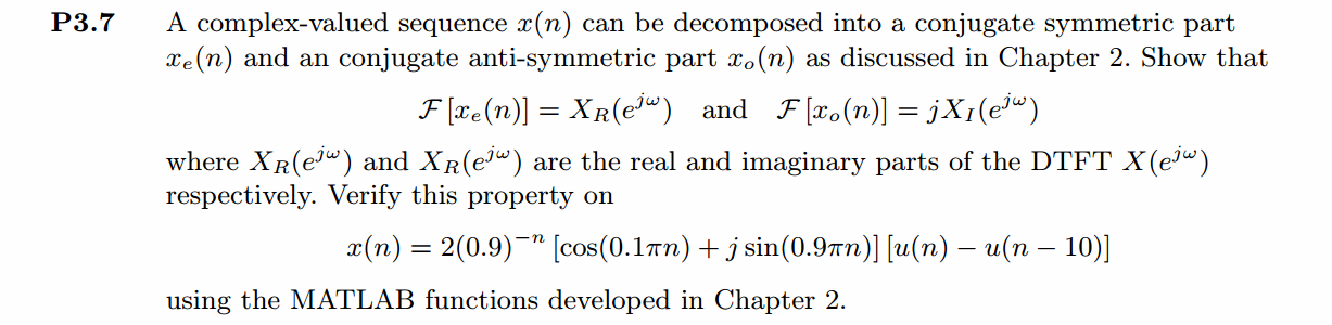
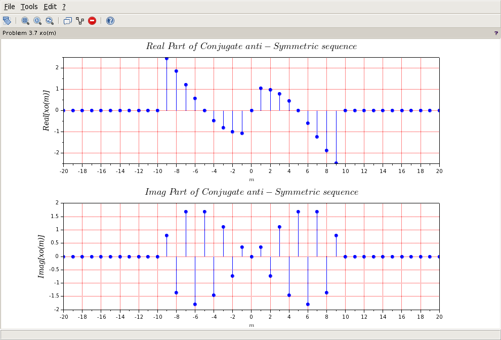
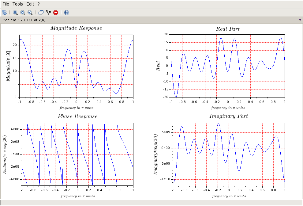
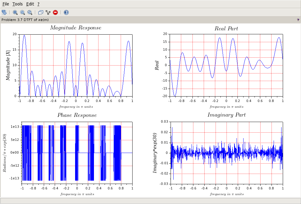
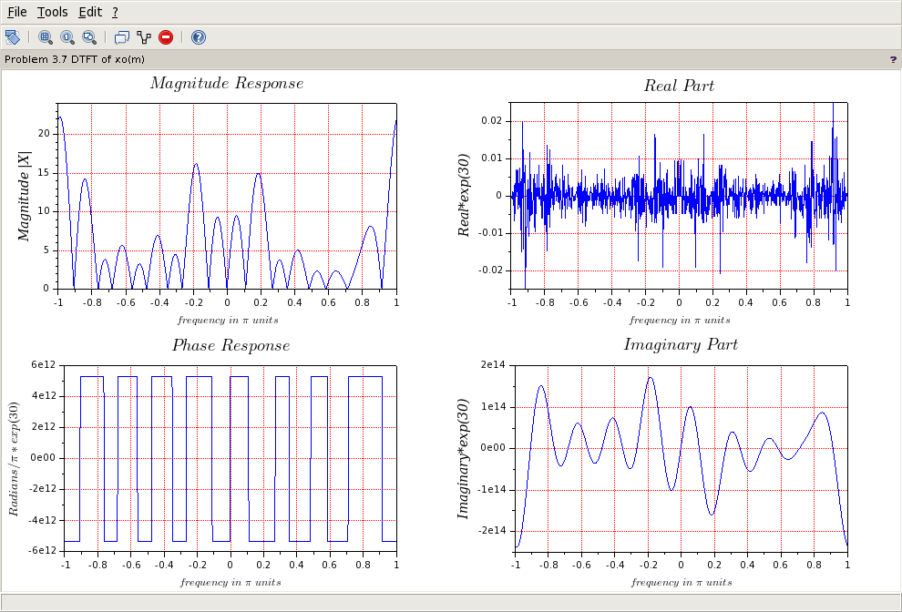
 一个复数序列x(n)可以分解为共轭对称序列xe(n)和共轭反对称序列xo(n)，各自对应的DTFT分别为X、XE、XO，则有：

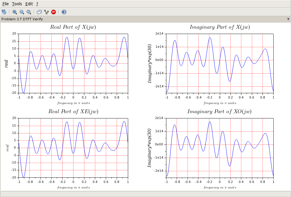
        （1）原始复序列的谱的实部（Real[X]）和共轭对称序列的谱的实部（Real[XE]）相同；

        （2）原始复序列的谱的虚部（Imag[X]）和共轭反对称序列的谱的虚部（Imag[XO]）相同；

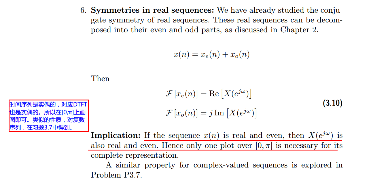
        （3）如果x(n)是实偶序列，则其DTFT也是实偶序列；

          前两个参照P3.7，第3个参照Example3.12。

一、上代码

// Book Author:Vinay K Ingle, John G Proakis
//
// Problem 3.7
// script by: KY
//
clear, clc, clf();

mode(2);
funcprot(0);
load('../fun/lib');

// -----------------------------------------------------------------------------
//                START        Output Info about this sce-file                 
mprintf('\n***********************************************************\n');
[ban1,ban2] = fun_banner();
mprintf("\n     <DSP using MATLAB> 3rd edition, Problem 3.7           \n");
mprintf(" ----------------------------------------------------------\n\n"); 

// ----------------END----------------------------------------------------------


n_start = -10; n_end = 20;
n = [n_start:n_end]; 
x = 2 * (0.9 .^(-n)) .* (cos(0.1*%pi*n) + %i*sin(0.9*%pi*n)) .* (fun_stepseq(0, n_start, n_end) - fun_stepseq(10, n_start, n_end)); 

[xe,xo,m] = fun_evenodd_cv(x,n);

// -----------------------------------------------------------------------------
// --------------------START  f0 figure-----------------------------------------
f0=scf(0);                    //creates figure with id==0 and make it the current one
  f0.figure_size=[1000,700];               // adjust window size
  f0.background=8;                         // add background color 8-white
  f0.figure_name="Problem 3.7 x(n)";      // name window
  subplot(2, 1, 1); 
     
     plot(n,real(x),'bo');
     plot(n,real(x),'b.');
  plot2d3(n,real(x),2);                        // Create plot with blue line
title("$Real\ Part\ of\ x(n)\ sequence$",'fontname',7,'fontsize',4);
//title("mprintf('x1(n) sequence, M = %d', M)");
xlabel('$n$','fontname',3); ylabel('Real[x(n)]','fontname',3,'fontsize',3);
xgrid(5,0,7);                             // color, thickness, style
a0=get("current_axes");                   // get the handle of the newly created axes
//a0.data_bounds=[-4,6,-6,6];

  subplot(2, 1, 2); 
     
     plot(n,imag(x),'bo');
     plot(n,imag(x),'b.');
  plot2d3(n,imag(x),2);                        // Create plot with blue line
title("$Imag\ Part\ of\ x(n)\ sequence$",'fontname',7,'fontsize',4);
//title("mprintf('x1(n) sequence, M = %d', M)");
xlabel('$n$','fontname',3); ylabel('Imag[x(n)]','fontname',3,'fontsize',3);
xgrid(5,0,7);                             // color, thickness, style
a1=get("current_axes");                   // get the handle of the newly created axes
//a1.data_bounds=[-4,6,-6,6];
// -----------------------------------------------------------------------------
// --------------------END  f0 -------------------------------------------------


// -----------------------------------------------------------------------------
// --------------------START  f1 figure-----------------------------------------
f1=scf(1);                    //creates figure with id==0 and make it the current one
  f1.figure_size=[1000,700];               // adjust window size
  f1.background=8;                         // add background color 8-white
  f1.figure_name="Problem 3.7 xe(m)";      // name window
  subplot(2, 1, 1); 
     
     plot(m,real(xe),'bo');
     plot(m,real(xe),'b.');
  plot2d3(m,real(xe),2);                        // Create plot with blue line
title("$Real\ Part\ of\ Conjugate-Symmetric\ sequence $",'fontname',7,'fontsize',4);
//title("mprintf('x1(n) sequence, M = %d', M)");
xlabel('$m$','fontname',3); ylabel('Real[xe(m)]','fontname',3,'fontsize',3);
xgrid(5,0,7);                             // color, thickness, style
a0=get("current_axes");                   // get the handle of the newly created axes
//a0.data_bounds=[-4,6,-6,6];

  subplot(2, 1, 2); 
     
     plot(m,imag(xe),'bo');
     plot(m,imag(xe),'b.');
  plot2d3(m,imag(xe),2);                        // Create plot with blue line
title("$Imag\ Part\ of\ Conjugate-Symmetric\ sequence$",'fontname',7,'fontsize',4);
//title("mprintf('x1(n) sequence, M = %d', M)");
xlabel('$m$','fontname',3); ylabel('Imag[xe(m)]','fontname',3,'fontsize',3);
xgrid(5,0,7);                             // color, thickness, style
a1=get("current_axes");                   // get the handle of the newly created axes
//a1.data_bounds=[-4,6,-6,6];
// -----------------------------------------------------------------------------
// --------------------END  f1 -------------------------------------------------


// -----------------------------------------------------------------------------
// --------------------START  f2 figure-----------------------------------------
f2=scf(2);                    //creates figure with id==0 and make it the current one
  f2.figure_size=[1000,700];               // adjust window size
  f2.background=8;                         // add background color 8-white
  f2.figure_name="Problem 3.7 xo(m)";      // name window
  subplot(2, 1, 1); 
     
     plot(m,real(xo),'bo');
     plot(m,real(xo),'b.');
  plot2d3(m,real(xo),2);                        // Create plot with blue line
title("$Real\ Part\ of\ Conjugate\ anti-Symmetric\ sequence $",'fontname',7,'fontsize',4);
//title("mprintf('x1(n) sequence, M = %d', M)");
xlabel('$m$','fontname',3); ylabel('Real[xo(m)]','fontname',3,'fontsize',3);
xgrid(5,0,7);                             // color, thickness, style
a0=get("current_axes");                   // get the handle of the newly created axes
//a0.data_bounds=[-4,6,-6,6];

  subplot(2, 1, 2); 
     
     plot(m,imag(xo),'bo');
     plot(m,imag(xo),'b.');
  plot2d3(m,imag(xo),2);                        // Create plot with blue line
title("$Imag\ Part\ of\ Conjugate\ anti-Symmetric\ sequence$",'fontname',7,'fontsize',4);
//title("mprintf('x1(n) sequence, M = %d', M)");
xlabel('$m$','fontname',3); ylabel('Imag[xo(m)]','fontname',3,'fontsize',3);
xgrid(5,0,7);                             // color, thickness, style
a1=get("current_axes");                   // get the handle of the newly created axes
//a1.data_bounds=[-4,6,-6,6];
// -----------------------------------------------------------------------------
// --------------------END  f2 -------------------------------------------------



//% ----------------------------------------------
//%           DTFT of x(n)
//% ----------------------------------------------

MM = 500;
k = [-MM:MM];        // [-pi, pi]
//%k = [0:M];        // [0, pi]
w = (%pi/MM) * k;

[X] = fun_dtft(x, n, w);                            

magX = abs(X); angX = fun_angle(X); realX = real(X); imagX = imag(X);

//%% ---------------------------------------------------------------------------
//%%                   START X(w)'s  mag ang real imag
// --------------------START  f3 figure-----------------------------------------
f3=scf(3);                    //creates figure with id==0 and make it the current one
  f3.figure_size=[1000,700];               // adjust window size
  f3.background=8;                         // add background color 8-white
  f3.figure_name="Problem 3.7 DTFT of x(n)";         // name window
  subplot(2, 2, 1); 
     plot(w/%pi,magX);
title("$Magnitude\ Response$",'fontname',7,'fontsize',4);
xlabel('$frequency\ in\ \pi\ units$','fontname',3); ylabel('Magnitude |X|','fontname',3,'fontsize',3);
xgrid(5,0,7);                             // color, thickness, style
a0=get("current_axes");                   // get the handle of the newly created axes
//a0.data_bounds=[-4,6,-6,6];

 subplot(2, 2, 3); 
     plot(w/%pi,angX/%pi*exp(20));
title("$Phase\ Response$",'fontname',7,'fontsize',4);
xlabel('$frequency\ in\ \pi\ units$','fontname',3); ylabel('$Radians/\pi*exp(20)$','fontname',3,'fontsize',3);
xgrid(5,1,7);                            // color, thickness, style
a1=get("current_axes");                  // get the handle of the newly created axes
//a1.data_bounds=[-4,6,-2,2];

 subplot(2, 2, 2); 
     plot(w/%pi,realX);
title("$Real\ Part$",'fontname',7,'fontsize',4);
xlabel('$frequency\ in\ \pi\ units$','fontname',3); ylabel('Real','fontname',3,'fontsize',3);
//xgrid();
xgrid(5,1,7);                           // color, thickness, style
a2=get("current_axes");                 // get the handle of the newly created axes
//a2.data_bounds=[-4,6,-2,2];

 subplot(2, 2, 4); 
     plot(w/%pi,imagX*exp(20));
title("$Imaginary\ Part$",'fontname',7,'fontsize',4);
xlabel('$frequency\ in\ \pi\ units$','fontname',3); ylabel('Imaginary*exp(20)','fontname',3,'fontsize',3);
//xgrid();
xgrid(5,1,7);                          // color, thickness, style
a3=get("current_axes");                // get the handle of the newly created axes
//a2.data_bounds=[-4,6,-2,2];
// ----------------------------END f3-------------------------------------------
//%%                   END X(w)'s  mag ang real imag
//%% ---------------------------------------------------------------------------




//% ---------------------------------------------------
//%                   DTFT of xe(m)
//% ---------------------------------------------------

MM = 500;
k = [-MM:MM];        // [-pi, pi]
//%k = [0:M];        // [0, pi]
w = (%pi/MM) * k;

[XE] = fun_dtft(xe, m, w);                            

magXE = abs(XE); angXE = fun_angle(XE); realXE = real(XE); imagXE = imag(XE);

//%% ---------------------------------------------------------------------------
//%%                   START X(w)'s  mag ang real imag
// --------------------START  f4 figure-----------------------------------------
f4=scf(4);                    //creates figure with id==0 and make it the current one
  f4.figure_size=[1000,700];               // adjust window size
  f4.background=8;                         // add background color 8-white
  f4.figure_name="Problem 3.7 DTFT of xe(m)";         // name window
  subplot(2, 2, 1); 
     plot(w/%pi,magXE);
title("$Magnitude\ Response$",'fontname',7,'fontsize',4);
xlabel('$frequency\ in\ \pi\ units$','fontname',3); ylabel('Magnitude |X|','fontname',3,'fontsize',3);
xgrid(5,0,7);                             // color, thickness, style
a0=get("current_axes");                   // get the handle of the newly created axes
//a0.data_bounds=[-4,6,-6,6];

 subplot(2, 2, 3); 
     plot(w/%pi,angXE/%pi*exp(30));
title("$Phase\ Response$",'fontname',7,'fontsize',4);
xlabel('$frequency\ in\ \pi\ units$','fontname',3); ylabel('$Radians/\pi*exp(30)$','fontname',3,'fontsize',3);
xgrid(5,1,7);                            // color, thickness, style
a1=get("current_axes");                  // get the handle of the newly created axes
//a1.data_bounds=[-4,6,-2,2];

 subplot(2, 2, 2); 
     plot(w/%pi,realXE);
title("$Real\ Part$",'fontname',7,'fontsize',4);
xlabel('$frequency\ in\ \pi\ units$','fontname',3); ylabel('Real','fontname',3,'fontsize',3);
//xgrid();
xgrid(5,1,7);                           // color, thickness, style
a2=get("current_axes");                 // get the handle of the newly created axes
//a2.data_bounds=[-4,6,-2,2];

 subplot(2, 2, 4); 
     plot(w/%pi,imagXE*exp(30));
title("$Imaginary\ Part$",'fontname',7,'fontsize',4);
xlabel('$frequency\ in\ \pi\ units$','fontname',3); ylabel('Imaginary*exp(30)','fontname',3,'fontsize',3);
//xgrid();
xgrid(5,1,7);                          // color, thickness, style
a3=get("current_axes");                // get the handle of the newly created axes
//a2.data_bounds=[-4,6,-2,2];
// ----------------------------END f4-------------------------------------------
//%%                   END XE(jw)'s  mag ang real imag
//%% ---------------------------------------------------------------------------



//% ---------------------------------------------------
//%                   DTFT of xo(m)
//% ---------------------------------------------------

MM = 500;
k = [-MM:MM];        // [-pi, pi]
//k = [0:M];        // [0, pi]
w = (%pi/MM) * k;

[XO] = fun_dtft(xo, m, w);                            

magXO = abs(XO); angXO = fun_angle(XO); realXO = real(XO); imagXO = imag(XO);

//%% ---------------------------------------------------------------------------
//%%                   START X(w)'s  mag ang real imag
// --------------------START  f5 figure-----------------------------------------
f5=scf(5);                    //creates figure with id==0 and make it the current one
  f5.figure_size=[1000,700];               // adjust window size
  f5.background=8;                         // add background color 8-white
  f5.figure_name="Problem 3.7 DTFT of xo(m)";         // name window
  subplot(2, 2, 1); 
     plot(w/%pi,magXO);
title("$Magnitude\ Response$",'fontname',7,'fontsize',4);
xlabel('$frequency\ in\ \pi\ units$','fontname',3); ylabel('Magnitude |X|','fontname',3,'fontsize',3);
xgrid(5,0,7);                             // color, thickness, style
a0=get("current_axes");                   // get the handle of the newly created axes
//a0.data_bounds=[-4,6,-6,6];

 subplot(2, 2, 3); 
     plot(w/%pi,angXO/%pi*exp(30));
title("$Phase\ Response$",'fontname',7,'fontsize',4);
xlabel('$frequency\ in\ \pi\ units$','fontname',3); ylabel('$Radians/\pi*exp(30)$','fontname',3,'fontsize',3);
xgrid(5,1,7);                            // color, thickness, style
a1=get("current_axes");                  // get the handle of the newly created axes
//a1.data_bounds=[-4,6,-2,2];

 subplot(2, 2, 2); 
     plot(w/%pi,realXO*exp(30));
title("$Real\ Part$",'fontname',7,'fontsize',4);
xlabel('$frequency\ in\ \pi\ units$','fontname',3); ylabel('Real*exp(30)','fontname',3,'fontsize',3);
//xgrid();
xgrid(5,1,7);                           // color, thickness, style
a2=get("current_axes");                 // get the handle of the newly created axes
//a2.data_bounds=[-4,6,-2,2];

 subplot(2, 2, 4); 
     plot(w/%pi,imagXO*exp(30));
title("$Imaginary\ Part$",'fontname',7,'fontsize',4);
xlabel('$frequency\ in\ \pi\ units$','fontname',3); ylabel('Imaginary*exp(30)','fontname',3,'fontsize',3);
//xgrid();
xgrid(5,1,7);                          // color, thickness, style
a3=get("current_axes");                // get the handle of the newly created axes
//a2.data_bounds=[-4,6,-2,2];
// ----------------------------END f5-------------------------------------------
//%%                   END XO(jw)'s  mag ang real imag
//%% ---------------------------------------------------------------------------



//% ------------------------------------------
//%             Verify
//% ------------------------------------------
//%% ---------------------------------------------------------------------------
//%%                   START X(w)'s  mag ang real imag
// --------------------START  f6 figure-----------------------------------------
f6=scf(6);                    //creates figure with id==0 and make it the current one
  f6.figure_size=[1000,700];               // adjust window size
  f6.background=8;                         // add background color 8-white
  f6.figure_name="Problem 3.7 DTFT Verify";         // name window
  subplot(2, 2, 1); 
     plot(w/%pi,realX);
title("$Real\ Part\ of\ X(jw)$",'fontname',7,'fontsize',4);
xlabel('$frequency\ in\ \pi\ units$','fontname',3); ylabel('real','fontname',3,'fontsize',3);
xgrid(5,0,7);                             // color, thickness, style
a0=get("current_axes");                   // get the handle of the newly created axes
//a0.data_bounds=[-4,6,-6,6];

 subplot(2, 2, 3); 
     plot(w/%pi,realXE);
title("$Real\ Part\ of\ XE(jw)$",'fontname',7,'fontsize',4);
xlabel('$frequency\ in\ \pi\ units$','fontname',3); ylabel('$real$','fontname',3,'fontsize',3);
xgrid(5,1,7);                            // color, thickness, style
a1=get("current_axes");                  // get the handle of the newly created axes
//a1.data_bounds=[-4,6,-2,2];

 subplot(2, 2, 2); 
     plot(w/%pi,imagX*exp(30));
title("$Imaginary\ Part\ of\ X(jw)$",'fontname',7,'fontsize',4);
xlabel('$frequency\ in\ \pi\ units$','fontname',3); ylabel('Imaginary*exp(30)','fontname',3,'fontsize',3);
//xgrid();
xgrid(5,1,7);                           // color, thickness, style
a2=get("current_axes");                 // get the handle of the newly created axes
//a2.data_bounds=[-4,6,-2,2];

 subplot(2, 2, 4); 
     plot(w/%pi,imagXO*exp(30));
title("$Imaginary\ Part\ of\ XO(jw)$",'fontname',7,'fontsize',4);
xlabel('$frequency\ in\ \pi\ units$','fontname',3); ylabel('Imaginary*exp(30)','fontname',3,'fontsize',3);
//xgrid();
xgrid(5,1,7);                          // color, thickness, style
a3=get("current_axes");                // get the handle of the newly created axes
//a2.data_bounds=[-4,6,-2,2];
// ----------------------------END f6-------------------------------------------
//%%                   END X(w)'s  mag ang real imag
//%% ---------------------------------------------------------------------------

二、运行结果

1、原始复数序列

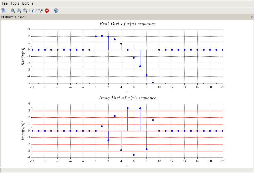
2、共轭对称序列xe

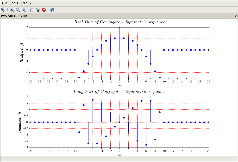
3、共轭反对称序列

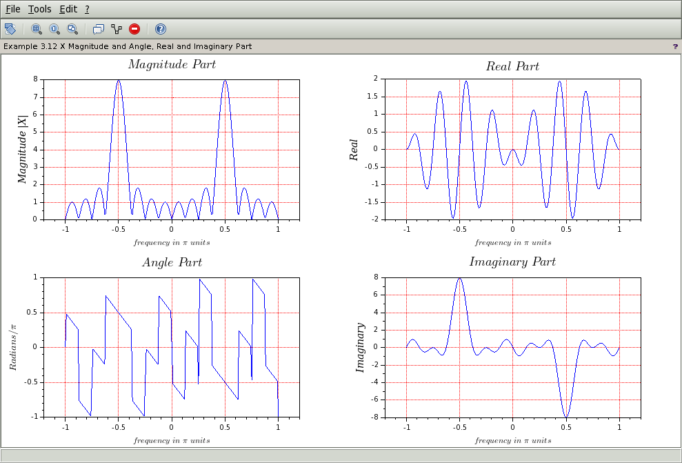
4、各自的DTFT

5、取出想要的图

 

一、上代码

// Book Author:Vinay K Ingle, John G Proakis
//
// Example 3.12
// script by: KY
//
clear, clc, clf();

mode(2);
funcprot(0);
//exec('fun_banner.sci');          // output version and OS info
//exec('fun_angle.sci');
//exec('fun_evenodd.sci');
load('../fun/lib');

// -----------------------------------------------------------------------------
//                START        Output Info about this sce-file                 
mprintf('\n***********************************************************\n');
[ban1,ban2] = fun_banner();
mprintf("\n     <DSP using MATLAB> 3rd edition, Example 3.12           \n");
mprintf(" ----------------------------------------------------------\n\n"); 

// ----------------END----------------------------------------------------------


n = -5:10; x = sin(%pi*n/2); 
k = -100:100; w = (%pi/100)*k;                // freqency between -pi and +pi  ,   [0,pi] axis divided into 101 points.
X = x * (exp(-%i*%pi/100)) .^ (n'*k);         // DTFT of x

// signal decomposition
[xe,xo,m] = fun_evenodd(x,n);                 // even and odd parts
XE = xe * (exp(-%i*%pi/100)) .^ (m'*k);       // DTFT of xe 
XO = xo * (exp(-%i*%pi/100)) .^ (m'*k);       // DTFT of xo 

magXE = abs(XE); angXE = fun_angle(XE); realXE = real(XE); imagXE = imag(XE);
magXO = abs(XO); angXO = fun_angle(XO); realXO = real(XO); imagXO = imag(XO);
magX  = abs(X);  angX  = fun_angle(X);  realX  = real(X);  imagX  = imag(X);

// verification
XR = real(X);                                  // real part of X
error1 = clean(max(abs(XE-XR)))                // Difference
XI = imag(X);                                  // imag part of X
error2 = clean(max(abs(XO-%i*XI)))             // Difference

// ------------START  f1 figure-------------------------------------------------
f1=scf(1);                    //creates figure with id==0 and make it the current one
  f1.figure_size=[900,700];                // adjust window size
  f1.background=8;                         // add background color 8-white
  f1.figure_name="Example 3.12 Fig1 x sequence";      // name window
  subplot(1, 1, 1); 
     plot(n,x,'bo');
     plot(n,x,'b.');
  plot2d3(n,x,2);                         // Create plot with blue line
title("$x\ sequence$",'fontname',7,'fontsize',4);
xlabel('$n$','fontname',3); ylabel('x(n)','fontname',3,'fontsize',3);
//xgrid();
xgrid(5,0,7);                             // color, thickness, style
a0=get("current_axes");                   // get the handle of the newly created axes
//a0.data_bounds=[0,13,0,1];
// -----------END f1------------------------------------------------------------


// ------------START  f2 figure-------------------------------------------------
f2=scf(2);                    //creates figure with id==0 and make it the current one
  f2.figure_size=[900,700];                // adjust window size
  f2.background=8;                         // add background color 8-white
  f2.figure_name="Example 3.12 Fig2 xe & xo sequence";      // name window
  subplot(2, 1, 1); 
     plot(m,xe,'bo');
     plot(m,xe,'b.');
  plot2d3(m,xe,2);                        // Create plot with blue line
title("$xe\ sequence$",'fontname',7,'fontsize',4);
xlabel('$n$','fontname',3); ylabel('xe(n)','fontname',3,'fontsize',3);
//xgrid();
xgrid(5,0,7);                             // color, thickness, style
a0=get("current_axes");                   // get the handle of the newly created axes
//a0.data_bounds=[0,13,0,1];

 subplot(2, 1, 2); 
     plot(m,xo,'bo');
     plot(m,xo,'b.');
  plot2d3(m,xo,2);                        // Create plot with blue line
title("$xo\ sequence$",'fontname',7,'fontsize',4);
xlabel('$n$','fontname',3); ylabel('xo(n)','fontname',3,'fontsize',3);
//xgrid();
xgrid(5,1,7);                             // color, thickness, style
a1=get("current_axes");                   // get the handle of the newly created axes
//a1.data_bounds=[0,13,0,1];
// -----------END f2------------------------------------------------------------


//%% ---------------------------------------------------------------------------
//%%                   START X's  mag ang real imag
// --------------------START  f3 figure-----------------------------------------
f3=scf(3);                    //creates figure with id==0 and make it the current one
  f3.figure_size=[1000,700];               // adjust window size
  f3.background=8;                         // add background color 8-white
  f3.figure_name="Example 3.12 X Magnitude and Angle, Real and Imaginary Part";         // name window
  subplot(2, 2, 1); 
     plot(w/%pi,magX);
title("$Magnitude\ Part$",'fontname',7,'fontsize',4);
xlabel('$frequency\ in\ \pi\ units$','fontname',3); ylabel('Magnitude |X|','fontname',3,'fontsize',3);
xgrid(5,0,7);                             // color, thickness, style
a0=get("current_axes");                   // get the handle of the newly created axes
//a0.data_bounds=[-4,6,-6,6];

 subplot(2, 2, 3); 
     plot(w/%pi,angX/%pi);
title("$Angle\ Part$",'fontname',7,'fontsize',4);
xlabel('$frequency\ in\ \pi\ units$','fontname',3); ylabel('$Radians/\pi$','fontname',3,'fontsize',3);
xgrid(5,1,7);                            // color, thickness, style
a1=get("current_axes");                  // get the handle of the newly created axes
//a1.data_bounds=[-4,6,-2,2];

 subplot(2, 2, 2); 
     plot(w/%pi,realX);
title("$Real\ Part$",'fontname',7,'fontsize',4);
xlabel('$frequency\ in\ \pi\ units$','fontname',3); ylabel('Real','fontname',3,'fontsize',3);
//xgrid();
xgrid(5,1,7);                           // color, thickness, style
a2=get("current_axes");                 // get the handle of the newly created axes
//a2.data_bounds=[-4,6,-2,2];

 subplot(2, 2, 4); 
     plot(w/%pi,imagX);
title("$Imaginary\ Part$",'fontname',7,'fontsize',4);
xlabel('$frequency\ in\ \pi\ units$','fontname',3); ylabel('Imaginary','fontname',3,'fontsize',3);
//xgrid();
xgrid(5,1,7);                          // color, thickness, style
a3=get("current_axes");                // get the handle of the newly created axes
//a2.data_bounds=[-4,6,-2,2];
// ----------------------------END f3-------------------------------------------
//%%                   END X's  mag ang real imag
//%% ---------------------------------------------------------------------------


//%% ---------------------------------------------------------------------------
//%%                   START XE's  mag ang real imag
// --------------------START  f4 figure-----------------------------------------
f4=scf(4);                    //creates figure with id==0 and make it the current one
  f4.figure_size=[1000,700];               // adjust window size
  f4.background=8;                         // add background color 8-white
  f4.figure_name="Example 3.12 XE Magnitude and Angle, Real and Imaginary Part";         // name window
  subplot(2, 2, 1); 
     plot(w/%pi,magXE);
title("$Magnitude\ Part$",'fontname',7,'fontsize',4);
xlabel('$frequency\ in\ \pi\ units$','fontname',3); ylabel('Magnitude |XE|','fontname',3,'fontsize',3);
xgrid(5,0,7);                             // color, thickness, style
a0=get("current_axes");                   // get the handle of the newly created axes
//a0.data_bounds=[-4,6,-6,6];

 subplot(2, 2, 3); 
     plot(w/%pi,angXE/%pi);
title("$Angle\ Part$",'fontname',7,'fontsize',4);
xlabel('$frequency\ in\ \pi\ units$','fontname',3); ylabel('$Radians/\pi$','fontname',3,'fontsize',3);
xgrid(5,1,7);                            // color, thickness, style
a1=get("current_axes");                  // get the handle of the newly created axes
//a1.data_bounds=[-4,6,-2,2];

 subplot(2, 2, 2); 
     plot(w/%pi,realXE);
title("$Real\ Part$",'fontname',7,'fontsize',4);
xlabel('$frequency\ in\ \pi\ units$','fontname',3); ylabel('Real','fontname',3,'fontsize',3);
//xgrid();
xgrid(5,1,7);                           // color, thickness, style
a2=get("current_axes");                 // get the handle of the newly created axes
//a2.data_bounds=[-4,6,-2,2];

 subplot(2, 2, 4); 
     plot(w/%pi,imagXE);
title("$Imaginary\ Part$",'fontname',7,'fontsize',4);
xlabel('$frequency\ in\ \pi\ units$','fontname',3); ylabel('Imaginary','fontname',3,'fontsize',3);
//xgrid();
xgrid(5,1,7);                          // color, thickness, style
a3=get("current_axes");                // get the handle of the newly created axes
//a2.data_bounds=[-4,6,-2,2];
// ----------------------------END f4-------------------------------------------
//%%                   END XE's  mag ang real imag
//%% ---------------------------------------------------------------------------


//%% ---------------------------------------------------------------------------
//%%                   START XO's  mag ang real imag
// --------------------START  f5 figure-----------------------------------------
f5=scf(5);                    //creates figure with id==0 and make it the current one
  f5.figure_size=[1000,700];               // adjust window size
  f5.background=8;                         // add background color 8-white
  f5.figure_name="Example 3.12 XO Magnitude and Angle, Real and Imaginary Part";         // name window
  subplot(2, 2, 1); 
     plot(w/%pi,magXO);
title("$Magnitude\ Part$",'fontname',7,'fontsize',4);
xlabel('$frequency\ in\ \pi\ units$','fontname',3); ylabel('Magnitude |XO|','fontname',3,'fontsize',3);
xgrid(5,0,7);                             // color, thickness, style
a0=get("current_axes");                   // get the handle of the newly created axes
//a0.data_bounds=[-4,6,-6,6];

 subplot(2, 2, 3); 
     plot(w/%pi,angXO/%pi);
title("$Angle\ Part$",'fontname',7,'fontsize',4);
xlabel('$frequency\ in\ \pi\ units$','fontname',3); ylabel('$Radians/\pi$','fontname',3,'fontsize',3);
xgrid(5,1,7);                            // color, thickness, style
a1=get("current_axes");                  // get the handle of the newly created axes
//a1.data_bounds=[-4,6,-2,2];

 subplot(2, 2, 2); 
     plot(w/%pi,realXO);
title("$Real\ Part$",'fontname',7,'fontsize',4);
xlabel('$frequency\ in\ \pi\ units$','fontname',3); ylabel('Real','fontname',3,'fontsize',3);
//xgrid();
xgrid(5,1,7);                           // color, thickness, style
a2=get("current_axes");                 // get the handle of the newly created axes
//a2.data_bounds=[-4,6,-2,2];

 subplot(2, 2, 4); 
     plot(w/%pi,imagXO);
title("$Imaginary\ Part$",'fontname',7,'fontsize',4);
xlabel('$frequency\ in\ \pi\ units$','fontname',3); ylabel('Imaginary','fontname',3,'fontsize',3);
//xgrid();
xgrid(5,1,7);                          // color, thickness, style
a3=get("current_axes");                // get the handle of the newly created axes
//a2.data_bounds=[-4,6,-2,2];
// ----------------------------END f5-------------------------------------------
//%%                   END XO's  mag ang real imag
//%% ---------------------------------------------------------------------------



// -----------------------------------------------------------------------------
//                    START Graphical verification
// -------------------START f6 figure------------------------------------------
f6=scf(6);                    //creates figure with id==0 and make it the current one
  f6.figure_size=[1000,700];                // adjust window size
  f6.background=8;                          // add background color 8-white
  f6.figure_name="Example 3.12 Fig6: Graphical verification";      // name window
  subplot(2, 2, 1); 
     plot(w/%pi,XR);
//     plot(w/%pi,magX);
//  plot2d3(n1,x1,2);                      // Create plot with blue line
title("$Real\ Part\ Of\ X$",'fontname',7,'fontsize',4);
xlabel('$frequency\ in\ \pi\ units$','fontname',3); ylabel('Re(X)','fontname',3,'fontsize',3);
//xgrid();
xgrid(5,0,7);                             // color, thickness, style
a0=get("current_axes");                   // get the handle of the newly created axes
//a0.data_bounds=[-4,6,-6,6];

 subplot(2, 2, 2); 
     plot(w/%pi,XI);
//     plot(n1,y1,'b.');
//  plot2d3(n1,y1,2);                      // Create plot with blue line
title("$Imaginary\ Part\ Of\ X$",'fontname',7,'fontsize',4);
xlabel('$frequency\ in\ \pi\ units$','fontname',3); ylabel('$Im(X)$','fontname',3,'fontsize',3);
//xgrid();
xgrid(5,1,7);                             // color, thickness, style
a1=get("current_axes");                   // get the handle of the newly created axes
//a1.data_bounds=[-4,6,-2,2];

 subplot(2, 2, 3); 
     plot(w/%pi,realXE);
//     plot(n1,y1,'b.');
//  plot2d3(n1,y1,2);                      // Create plot with blue line
title("$Transform\ of\ even\ part$",'fontname',7,'fontsize',4);
xlabel('$frequency\ in\ \pi\ units$','fontname',3); ylabel('$XE$','fontname',3,'fontsize',3);
//xgrid();
xgrid(5,1,7);                             // color, thickness, style
a2=get("current_axes");                   // get the handle of the newly created axes
//a2.data_bounds=[-4,6,-2,2];

 subplot(2, 2, 4); 
     plot(w/%pi,imagXO);
//     plot(n1,y1,'b.');
//  plot2d3(n1,y1,2);                      // Create plot with blue line
title("$Transform\ of\ odd\ part$",'fontname',7,'fontsize',4);
xlabel('$frequency\ in\ \pi\ units$','fontname',3); ylabel('$XO$','fontname',3,'fontsize',3);
//xgrid();
xgrid(5,1,7);                             // color, thickness, style
a3=get("current_axes");                   // get the handle of the newly created axes
//a2.data_bounds=[-4,6,-2,2];
// ------------------------END f6-----------------------------------------------
//                  END Y's  mag ang real imag
// -----------------------------------------------------------------------------

二、运行结果

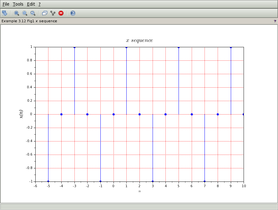
1、原始实数序列

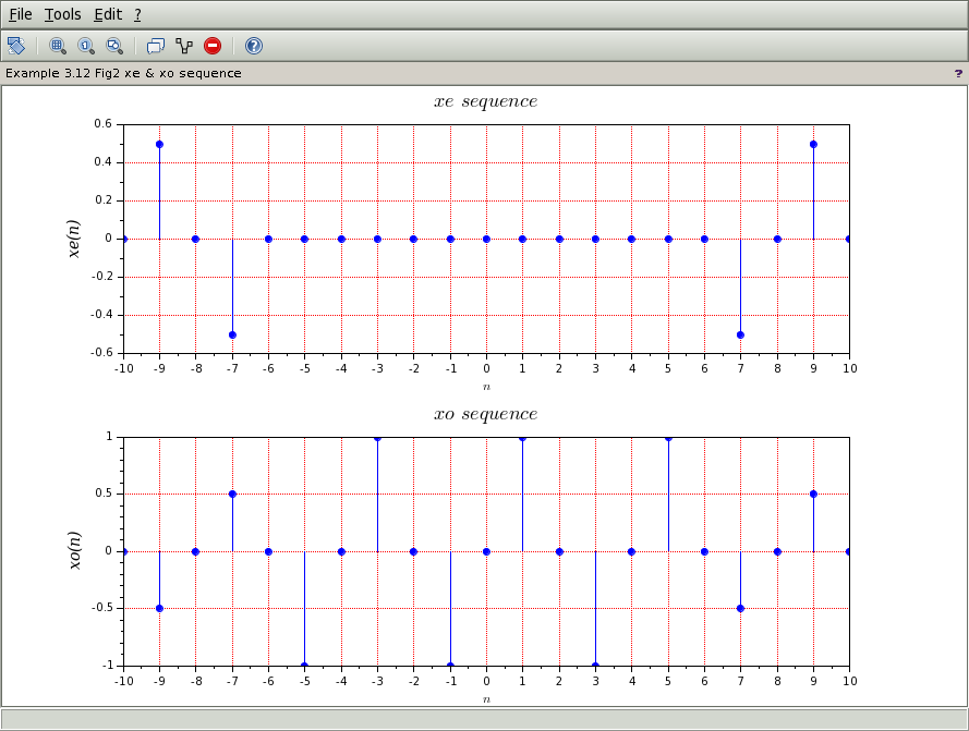
2、分解成偶序列和奇序列。

3、这里只放x的DTFT，其奇偶分解序列的DTFT就不放了

 

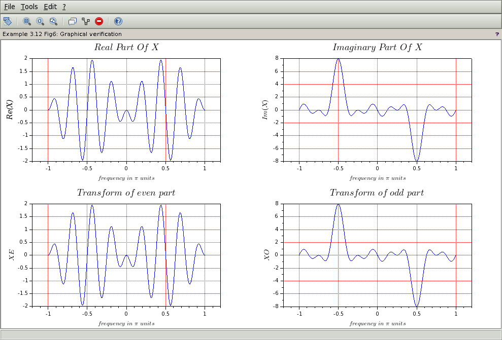
        至此，博文开头有关对称性（Symmetriy）性质的3条就都用图形来表达了。