Approximation Theory and Method part 2

Approximation Theory and Method part 2

Approximation operators

在前面的讨论中，我们得到了 best approximation 的一些性质. 但是实际上我们并不总是能有 best approximation 这么好的结果。那么我们能不能退而求其次，研究一下更具一般性的 approximation operators 呢？

We note that the operator \(\boldsymbol X\) is defined to be a projection if the equation

\[\boldsymbol{X}[\boldsymbol{X}(f)]=\boldsymbol{X}(f), \quad f \in \mathscr{B}, \]

is satisfied. Hence a sufficient condition for \(X\) to be a projection is the equation

\[X(a)=a, \quad a \in \mathscr{A} \]

Most of the approximation methods that are considered in this book do satisfy condition (3.2), but an important exception is the Bernstein operator, which is discussed in Chapter 6. Sometimes \(X(f)\) is written as \(X f\).

The idea of a linear operator is also well known; namely, we define \(X\) to be linear if the equation

\[X(\lambda f)=\lambda \boldsymbol{X}(f) \]

holds for all \(f \in \mathscr{B}\), where \(\lambda\) is any real number, and if the equation

\[\boldsymbol{X}(f+g)=\boldsymbol{X}(f)+\boldsymbol{X}(g) \]

is obtained for all \(f \in \mathscr{B}\) and for all \(g \in \mathscr{B}\).

最好还是定义一下这些 approximation operator 的 norm.

Also we make frequent use of the norm of an approximation operator. The norm of \(X\) is written as \(\|X\|\), and it is the smallest real number such that the inequality

\[\|\boldsymbol{X}(f)\| \leqslant\|\boldsymbol{X}\|\|f\| \]

或者可以这样写

\[\|\boldsymbol{X} \| = \sup _{ \|f\| \neq 0} \frac{\|\boldsymbol{X}(f)\| }{\|f\|} \]

这和我们定义矩阵时是类似的. 比如矩阵\(A\) 的 norm:

\[\|A \| = \sup _{ \|x\| \neq 0} \frac{\|Ax\| }{\|x\|} \]

关于 norm of approximation operator 的取值问题，可以考虑一个例子.

An example of an approximation operator that is useful because it is easy to apply is as follows. Let \(\mathscr{B}\) be the space \(\mathscr{C}[0,1]\) of real-valued functions that are continuous on \([0,1]\), and let \(\mathscr{A}\) be the linear space \(\mathscr{P}_1\) of all real polynomials of degree at most one. Then, in order that the calculation of an approximation to a function \(f\) in \(\mathscr{R}\) depends on only two function evaluations, we let \(p\) be the polynomial in \(\mathscr{A}\) that satisfies the interpolation conditions

\[\left.\begin{array}{l} p(0)=f(0) \\ p(1)=f(1) \end{array}\right\} \]

Thus \(p=X(f)\), where \(X\) is a linear projection operator from \(\mathscr{B}\) to \(\mathscr{A}\).
In order to define the norm of this operator we choose a norm for the space \(\mathscr{C}[0,1]\). However, if the 2-norm

\[\|f\|_2=\left\{\int_0^1[f(x)]^2 \mathrm{~d} x\right\}^{\frac{1}{2}}, \quad f \in \mathscr{C}[0,1], \]

is used, we find that the operator \(X\) is unbounded, because it is possible for \(\|X f\|_2\) to be one when \(\|f\|_2\) is arbitrarily small. It is therefore necessary to prefer the \(\infty\)-norm

\[\|f\|_{\infty}=\max _{0 \leqslant x \leqslant 1}|f(x)|, \quad f \in \mathscr{C}[0,1] \]

when considering approximation operators that are defined by interpolation conditions. In this case, because \(p\) is in \(\mathscr{P}_1\), equation (3.6) implies the inequality

\[\begin{aligned} \|X(f)\| & =\|p\| \\ & =\max [|p(0)|,|p(1)|] \\ & =\max [|f(0)|,|f(1)|] \\ & \leqslant\|f\|, \quad f \in \mathscr{C}[0,1] . \end{aligned} \]

在这个例子中，我们的 approximation operator 可以理解为把 0 和 1 处，也就是函数的两端进行连线. 可以发现此时 2-norm 可以去到很大，而 inf-norm 是有上确界的.

Lebesgue constants

Theorem 3.1
Let \(\mathscr{A}\) be a finite-dimensional linear subspace of a normed linear space \(\mathscr{B}\), and let \(X\) be a linear operator from \(\mathscr{B}\) to \(\mathscr{A}\) that satisfies the projection condition (3.2). For any \(f\) in \(\mathscr{B}\), let \(d^*\) be the least distance

\[d^*=\min _{a \in \mathbb{A}}\|f-a\| \]

from \(f\) to an element of \(\mathscr{A}\). Then the error of the approximation \(X(f)\) satisfies the bound

\[\|f-X(f)\| \leqslant[1+\|X\|] d^* \]

在上面我们退而求其次，使用一个满足 projection 和 linearity 的 approximation operator 来进行逼近. 感觉这个逼近的结果和最优点有一段距离，在这里定理3.1 给出了一个上界: 肯定在最优附近的\([1+\|X\|]\)范围内.

Polynomial approximations to differentiable functions

在后面我们会证明，对于任意一个函数\(f \in \mathscr{C}[a, b]\)，我们可以用多项式\(p\)进行逼近，并且可以让误差要多小有多小.

\[\|f-p\|_{\infty} \leqslant \varepsilon \]

看起来这是一个很强，而且不错的结果.

Polynomial interpolation

所谓多项式插值，就是对多项式进行一个值的插（）

比如有 \((n + 1)\) 组观测到的数据: \((x_i, y_i)\) for \(i = 0,1,...,n\), 实际上背后的函数是\(f\), 这个函数是什么函数都可以. 比如城市气温的函数, 我们想用多项式\(p\)进行逼近. 按照经验来看，比如我们有两个观测点，那我们能唯一确定一个 \(p \in \mathscr P_1\), 如果有5个观测点，那用那我们能唯一确定一个 \(p \in \mathscr P_4\).

关于\(\mathscr P_n\), 我们知道\(n\)是多项式的最高次数. 比如 \(p = 1+x\) 那么 \(p \in \mathscr P _1\), \(p = 1\) 那么 \(p \in \mathscr P_0\)

那多项式 \(p = 0\) 是几次多项式呢？

可以考虑 \(p = 0\) 的性质. 假设 \(p \in \mathscr P_?\) 假设有个 \(q \in \mathscr P_{4}\), \(pq = 0\) 所以 \(pq \in \mathscr P_{?}\).

所以感觉 \(? = - \infty\) 蛮不错. 那就定义成 \(p \in \mathscr P_{-\infty}\) .

希望在观测的地方，多项式的值就是实际函数的值. 那么这实际上就是一个解方程的问题：

\[\left\{\begin{array}{c} \sum c_i x_0^i=y_0 \\ \sum c_i x_1^i=y_1 \\ \vdots \\ \sum c_i x_n^i=y_n \end{array}\right. \]

想要知道这个方程组解的数量，实际上就是想知道 \(\det(V)\), where \(V\) is the Vandermonde matrix

\[V=V\left(x_0, x_1, \cdots, x_m\right)=\left[\begin{array}{ccccc} 1 & x_0 & x_0^2 & \ldots & x_0^n \\ 1 & x_1 & x_1^2 & \ldots & x_1^n \\ 1 & x_2 & x_2^2 & \ldots & x_2^n \\ \vdots & \vdots & \vdots & \ddots & \vdots \\ 1 & x_m & x_m^2 & \ldots & x_m^n \end{array}\right] \]

The determinant of a square Vandermonde matrix is called a Vandermonde polynomial or Vandermonde determinant. Its value is the polynomial

\[\operatorname{det}(V)=\prod_{0 \leq i<j \leq n}\left(x_j-x_i\right) \]

我们的假设是每个观测的点都不一样，所以 \(\operatorname{det}(V) \neq 0\). 也就是有唯一解.

在引入 Lagrange interpolation 之前，其实这个思想和中国剩余定理很相似. 不妨先复习复习中国剩余定理.

有物不知其数，三三数之剩二，五五数之剩三，七七数之剩二。问物几何？

也就是求解同余方程组:

\[\left\{\begin{aligned} x & \equiv 2 \quad\left(\bmod 3\right) \\ x & \equiv 3 \quad\left(\bmod 5\right) \\ x & \equiv 2 \quad \left(\bmod 7\right) \end{aligned}\right. \]

我们想知道，解的

• existence
• uniqueness
• how to find

首先确定解的范围. 可以注意到，如果 \(n_1\) 是一个解，那么 \(n_2 = n_1 + 105\) 也是一个可行解. 那么只考虑 \(R = [1, 105]\) 中的可行解就行了.

如果 \(n_1,n_2 \in R\) 是两个不同的解, 那么\(n_1 - n_2\) 一定被 3, 5, 7 整除，但是注意到 \(-104 \leq n_1 - n_2 \leq 104\)，这样的 \(n_1,n_2\) 并不存在. 所以，如果有在 \(R\) 中的解，这个解是唯一的.

关于存在性, 考虑问题集：

\[\left\{\begin{aligned} x & \equiv 0,1,2 \quad\left(\bmod 3\right) \\ x & \equiv 0,1,2,3,4 \quad\left(\bmod 5\right) \\ x & \equiv 0,1,2,3,4,5,6 \quad \left(\bmod 7\right) \end{aligned}\right. \]

意思是，在 \(\mod{}\) 后面的数字确定的情况下，一共有\(3\times 5 \times 7 = 105\) 个可能的问题. 可能的解有 \(|R| = 105\) 个, 每个问题的解都是唯一的, 不同问题的解肯定不一样，所以每个问题都有唯一解.

最后考虑怎么找到解. 我们采取分治思想，把原问题分成互不相干的若干子问题，每个子问题都相对好求解. 最后把子问题的解合并起来就得到原问题的解.

我们首先求解每个子问题：

\[\left\{\begin{aligned} x & \equiv 1 \quad\left(\bmod 3\right) \\ x & \equiv 0 \quad\left(\bmod 5\right) \\ x & \equiv 0 \quad \left(\bmod 7\right) \end{aligned}\right. \quad \left\{\begin{aligned} x & \equiv 0 \quad\left(\bmod 3\right) \\ x & \equiv 1 \quad\left(\bmod 5\right) \\ x & \equiv 0 \quad \left(\bmod 7\right) \end{aligned}\right. \quad \left\{\begin{aligned} x & \equiv 0 \quad\left(\bmod 3\right) \\ x & \equiv 0 \quad\left(\bmod 5\right) \\ x & \equiv 1 \quad \left(\bmod 7\right) \end{aligned}\right. \]

通俗地讲就是求每一行式子的乘法逆元. 乘法逆元可以用 extended Euclidean algorithm 来求. 在这个问题中，上面三个子问题对应的解是 \(70,21,15\). 这三个数字构成了问题集的解的线性基底，对于上述提到的 \(105\) 个可能的问题，每个问题都是这个线性基底的线性组合. 比如在这里就是 \((2\cdot 70 + 3 \cdot 21 + 2\cdot 15) \mod 105\).

The Lagrange interpolation formula

回到这个问题本身. 类似于刚刚的思想, 我们希望找到一组多项式 \(p_0, p_1, ... ,p_n\) 一共 \(n +1\) 个多项式，让每一个多项式 \(p_k(x)\) 在「自己负责的」采样点 \(x_k\) 处满足 \(p(x_k) = 1\), 在其他地方 \(p(x_i) = 0(i\neq k)\).

这样一来对于任意一个函数 \(f\), 对于固定的采样点集合，我们都可以用上述的一组多项式基底来线性合成一个关于 \(f\) 的多项式逼近.

For \(k=0,1, \ldots, n\), let \(l_k\) be the function

\[l_k(x)=\prod_{\substack{j=0 \\ j \neq k}}^n\left(x-x_j\right) /\left(x_k-x_j\right), \quad a \leqslant x \leqslant b . \]

We note that \(l_k \in \mathscr{P}_n\) and that the equations

\[l_k\left(x_i\right)=\delta_{k i}, \quad i=0,1, \ldots, n, \]

hold, where \(\delta_{k i}\) has the value

\[\delta_{k i}= \begin{cases}1, & k=i \\ 0, & k \neq i\end{cases} \]

Polynomial interpolation
It follows that the function

\[p=\sum_{k=0}^n f\left(x_k\right) l_k \]

\[p(x)=\sum_{k=0}^n f\left(x_k\right) l_k(x) . \]

This method is called the Lagrange interpolation formula.

Properties

We can regrard the Lagrange interplation process as an operator from \(\mathscr C [a,b]\) to \(\mathscr P_n\). The operator is

• a projection
• linear

The error in polynomial interpolation

We use the notation \(e\) for the error function of an approximation, and in this chapter it has the value

\[e(x)=f(x)-p(x), \quad a \leqslant x \leqslant b \]

where \(p\) is the polynomial in \(\mathscr{P}_n\) that satisfies the interpolation conditions (4.2). It should be clear that, if we change \(f\) by adding to it an element of \(\mathscr{P}_n\), then the interpolation process automatically adds the same element to \(p\), which leaves \(e\) unchanged. Expressions for the error should show this property. It is therefore appropriate, when \(f \in \mathscr{C}^{(n+1)}[a, b]\), to state \(e\) in terms of the derivative \(f^{(n+1)}\), which is done in our next theorem.
Theorem 4.2
For any set of distinct interpolation points \(\left\{x_i ; i=0,1, \ldots, n\right\}\) in \([a, b]\) and for any \(f \in \mathscr{C}^{(n+1)}[a, b]\), let \(p\) be the element of \(\mathscr{P}_n\) that satisfies the equations (4.2). Then, for any \(x\) in \([a, b]\), the error (4.12) has the value

\[e(x)=\frac{1}{(n+1) !} \prod_{j=0}^n\left(x-x_j\right) f^{(n+1)}(\xi) \]

where \(\xi\) is a point of \([a, b]\) that depends on \(x\).

可以看到，误差的来源和

• 采样点的位置
• \(f\) 本身
• 采样点的数量

有关.

Runge's phenomenon

感觉上，采样点越多，误差应该越小才对. 可是事实上不是这样，如果我们只是简单均匀采样，多项式的误差并不会越来越小.

\[f(x)=1 /\left(1+x^2\right), \quad-5 \leqslant x \leqslant 5 \]

n	\(f\left(x_{n-\frac{1}{2}}\right)\)	\(p\left(x_{n-\frac{1}{2}}\right)\)	\(e\left(x_{n-\frac{1}{2}}\right)\)
2	0.137931	0.759615	-0.621684
4	0.066390	-0.356826	0.423216
6	0.054463	0.607879	-0.553416
8	0.049651	-0.831017	0.880668
10	0.047059	1.578721	-1.531662
12	0.045440	-2.755000	2.800440
14	0.044334	5.332743	-5.288409
16	0.043530	-10.173867	10.217397
18	0.042920	20.123671	-20.080751
20	0.042440	-39.952449	39.994889

误差在变大?

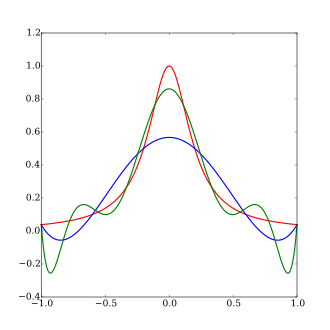
图源维基百科. 和数据无关.

The Chebyshev interpolation points

用这个方法解决采样位置不好导致的误差变大问题.

Theorem 4.3
The norm of the Lagrange interpolation operator has the value

\[\|\boldsymbol{X}\|=\max _{a \leqslant x \leqslant b} \sum_{k=0}^n\left|l_k(x)\right| \]

where the functions \(\left\{l_k ; k=0,1, \ldots, n\right\}\) are defined by equation (4.3).
Proof. The definition of a norm and equation (4.6) give the identity

\[\begin{aligned} \|\boldsymbol{X}\| & =\sup _{\|f\| \leqslant 1}\|\boldsymbol{X}(f)\| \\ & =\sup _{\|f\| \leqslant 1} \max _{a \leqslant x \leqslant b}\left|\sum_{k=0}^n f\left(x_k\right) l_k(x)\right| \\ & =\max _{a \leqslant x \leqslant b} \sup _{\|f\| \leqslant 1} \left|\sum_{k=0}^n f\left(x_k\right) l_k(x)\right| \\ & =\max _{a \leqslant x \leqslant b} \sum_{k=0}^n\left|l_k(x)\right| \end{aligned} \]

which is the required result.

解释解释每一个等号都是为什么：

The first quality: Consider the definition of norm of approximation operator: The norm of \(X\) is written as \(\|X\|\), and it is the smallest real number such that the inequality \(\|\boldsymbol{X}(f)\| \leqslant\|\boldsymbol{X}\|\|f\|\) holds. Here, if \(\| f \|\) is not equal to one, then suppose \(\| f \| = a \neq 0\), Then

Left hand side:

\[\begin{aligned} \|\boldsymbol{X}((1/a)f)\| &= \|(1/a)\boldsymbol{X}(f)\| \quad \text{the approximation operator of Lagrange interpolation is linear}\\ &= |(1/a)|\cdot \|\boldsymbol{X}(f)\| \quad \text{absolute homogeneity of norm} \end{aligned} \]

Right hand side:

\[\|\boldsymbol{X}\|\| (1/a)f \| = |(1/a)|\cdot \|\boldsymbol{X}\|\|f \|\quad \text{absolute homogeneity of norm} \]

That is, \(|(1/a)|\) appears on both the LHS and RHS of \(\|\boldsymbol{X}(f)\| \leqslant\|\boldsymbol{X}\|\|f\|\) when \(\| f \| \neq 1\), it can thus be cancelled out.

So

\[\begin{aligned} \|\boldsymbol{X} \| &= \sup _{ \|f\| \neq 0} \frac{\|\boldsymbol{X}(f)\| }{\|f\|} \\ &= \sup _{\|f\| = 1} \frac{\|\boldsymbol{X}(f)\| }{\|f\|} \\ &= \sup _{\|f\| = 1} \|\boldsymbol{X}(f)\| \\ &= \sup _{\|f\| \leq 1} \|\boldsymbol{X}(f)\| \end{aligned} \]

The second equality: this is by the definition of infinity norm.

The third equality:

Theorem (supremum of supremum is interchangeable)

\[\sup _{a \in A} \sup _{b \in B} F(a, b)=\sup _{(a, b) \in A \times B} F(a, b)=\sup _{b \in B} \sup _{a \in A} F(a, b) \]

Let us prove the first equality and the second follows symmetrically.
Let \(S_1=\sup _{a \in A} \sup _{b \in B} F(a, b)\) and \(S_2=\sup _{(a, b) \in A \times B} F(a, b)\). Suppose that \(S_1<S_2\). Then, since \(S_2\) is the least upper bound of the set \(\{F(a, b):(a, b) \in A \times B\}\), there exist \(\left(a_0, b_0\right) \in A \times B\) with \(S_1<F(a, b)\). But then

\[F\left(a_0, b_0\right) \leq \sup _{b \in B} F\left(a_0, b\right) \leq \sup _{a \in A} \sup _{b \in B} F(a, b)=S_1 \]

a contradiction.
Next, suppose that \(S_2<S_1\). Then, because \(S_1\) is the least upper bound of \(\left\{\sup _{b \in B} F(a, b): a \in A\right\}\), it follows that there is some \(a_0 \in A\) such that \(S_2<\sup _{b \in B} F\left(a_0, b\right)\). Similarly, there now exists \(b_0 \in B\) such that \(S_2<F\left(a_0, b_0\right)\), a contradiction. \(\square\)

Here, \(\left|\sum_{k=0}^n f\left(x_k\right) l_k(x)\right|\) is continuous and is defined on a closed interval, so \(\max _{a \leqslant x \leqslant b}\left|\sum_{k=0}^n f\left(x_k\right) l_k(x)\right| = \sup _{a \leqslant x \leqslant b}\left|\sum_{k=0}^n f\left(x_k\right) l_k(x)\right|\).

Then

\[\begin{aligned} &\sup _{\|f\| \leqslant 1} \max _{a \leqslant x \leqslant b}\left|\sum_{k=0}^n f\left(x_k\right) l_k(x)\right| \\ =&\sup _{\|f\| \leqslant 1} \sup _{a \leqslant x \leqslant b}\left|\sum_{k=0}^n f\left(x_k\right) l_k(x)\right| \\ =&\sup _{a \leqslant x \leqslant b} \sup _{\|f\| \leqslant 1} \left|\sum_{k=0}^n f\left(x_k\right) l_k(x)\right| \\ =&\max _{a \leqslant x \leqslant b} \sup _{\|f\| \leqslant 1} \left|\sum_{k=0}^n f\left(x_k\right) l_k(x)\right| \\ \end{aligned} \]

The fourth equality: when \(f(x_k) = 1\) for all \(k\), $\left|\sum_{k=0}^n f\left(x_k\right) l_k(x)\right| $ reaches its maximum. Since \(\|f\| \leqslant 1\) is a closed constraint, this is also its supremum.

Recall that

Theorem 3.1
Let \(\mathscr{A}\) be a finite-dimensional linear subspace of a normed linear space \(\mathscr{B}\), and let \(X\) be a linear operator from \(\mathscr{B}\) to \(\mathscr{A}\) that satisfies the projection condition (3.2). For any \(f\) in \(\mathscr{B}\), let \(d^*\) be the least distance

\[d^*=\min _{a \in \mathbb{A}}\|f-a\| \]

from \(f\) to an element of \(\mathscr{A}\). Then the error of the approximation \(X(f)\) satisfies the bound

\[\|f-\boldsymbol{X}(f)\| \leqslant[1+\|\boldsymbol{X}\|] d^* \]

我们想知道 \(\| \boldsymbol X \|\) 好不好，至少想知道他至少是多少. 上面他做了一些实验，我们可以用观测到的数据给出 \(\| \boldsymbol X \|\) 的一个下界.

\[\begin{aligned} \|\boldsymbol{X}\| &\geq \frac{\|f-\boldsymbol{X}(f)\| }{d^*} - 1 \\ & \geq \frac{\max \left|f(x_i)-\boldsymbol{X}(f(x_i))\right|}{d^{*+}} \\ & = (39.994889 / 0.015507)-1 =10 986.71 \end{aligned} \]

还是蛮大的，毕竟 \(\boldsymbol X\) 只说了是从什么东西映射到了什么东西，没说采样的时候是怎样采样，所以可以相当大. 所以我们在采样的时候要选择比较安全的方式，比如使用 Chebyshev interpolation points.

但是要注意，Chebyshev interpolation points 并不是万金油，尽管使用了这种方法，误差也相当大的情况依然存在.