Python for Data Science - Principal component analysis (PCA)

Chapter 5 - Dimensionality Reduction Methods

Segment 2 - Principal component analysis (PCA)

Singular Value Decomposition

A linear algebra method that decomposes a matrix into three resultant matrices in order to reduce information redundancy and noise

SVD is most commonly used for principal component analysis.

The Anatomy of SVD

A = u * v * S

• A = Original matrix
• u = Left orthogonal matrix: hold important, nonredundant information about observations
• v = Right orthogonal matrix: holds important, nonredundant information on features
• S = Diagonal matrix: contains all of the information about the decomposition processes performed during the compression

Principal Component

Uncorrelated features that embody a dataset's important information (its "variance") with the redundancy, noise, and outliers stripped out

PCA Use Cases

• Fraud Detection
• Speech Recognition
• Spam Detection
• Image Recognition

Using Factors and Components

• Both factors and components represent what is left of a dataset after information redundancy and noise is stripped out
• Use them as input variables for machine learning algorithms to generate predictions from these compressed representations of your data

import numpy as np
import pandas as pd

import matplotlib.pyplot as plt
import pylab as plt
import seaborn as sb
from IPython.display import Image
from IPython.core.display import HTML 
from pylab import rcParams

import sklearn
from sklearn import datasets

from sklearn import decomposition
from sklearn.decomposition import PCA

%matplotlib inline
rcParams['figure.figsize'] = 5, 4
sb.set_style('whitegrid')

PCA on the iris dataset

iris = datasets.load_iris()
X = iris.data
variable_names = iris.feature_names

X[0:10,]

array([[5.1, 3.5, 1.4, 0.2],
       [4.9, 3. , 1.4, 0.2],
       [4.7, 3.2, 1.3, 0.2],
       [4.6, 3.1, 1.5, 0.2],
       [5. , 3.6, 1.4, 0.2],
       [5.4, 3.9, 1.7, 0.4],
       [4.6, 3.4, 1.4, 0.3],
       [5. , 3.4, 1.5, 0.2],
       [4.4, 2.9, 1.4, 0.2],
       [4.9, 3.1, 1.5, 0.1]])

pca = decomposition.PCA()
iris_pca = pca.fit_transform(X)

pca.explained_variance_ratio_

array([0.92461872, 0.05306648, 0.01710261, 0.00521218])

pca.explained_variance_ratio_.sum()

1.0

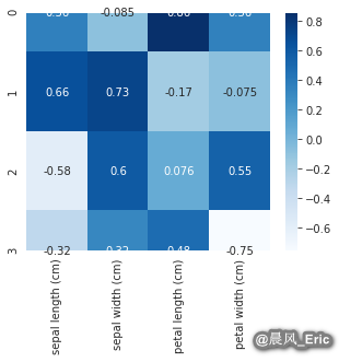
comps = pd.DataFrame(pca.components_, columns=variable_names)
comps

	sepal length (cm)	sepal width (cm)	petal length (cm)	petal width (cm)
0	0.361387	-0.084523	0.856671	0.358289
1	0.656589	0.730161	-0.173373	-0.075481
2	-0.582030	0.597911	0.076236	0.545831
3	-0.315487	0.319723	0.479839	-0.753657

sb.heatmap(comps,cmap="Blues", annot=True)

<matplotlib.axes._subplots.AxesSubplot at 0x7f436793d240>