

目录
一、Load Data 加载数据
1.数据解释
| Variable | Description | Transformation |
|---|---|---|
| realgdp | Real gross domestic product(实际国内生产总值) | Annual Growth Rate(年增长率) |
| realcons | Real personal consumption expenditures(实际个人消费支出) | Annual Growth Rate(年增长率) |
| realinv | Real gross private domestic investment(实际私人国内总投资) | Annual Growth Rate(年增长率) |
| realgovt | Real federal expenditures & gross investment(实际联邦政府支出与总投资) | Annual Growth Rate(年增长率) |
| realdpi | Real private disposable income(实际私人可支配收入) | Annual Growth Rate(年增长率) |
| m1 | M1 nominal money stock(名义M1货币供应量) | Annual Growth Rate(年增长率) |
| tbilrate | Monthly treasury bill rate(月度国库券利率) | Level(水平值) |
| unemp | Seasonally adjusted unemployment rate (%)(季调失业率,单位:%) | Level(水平值) |
| infl | Inflation rate(通货膨胀率) | Level(水平值) |
| realint | Real interest rate(实际利率) | Level(水平值) |
通过
import statsmodels.api as sm
data = pd.DataFrame(sm.datasets.macrodata.load().data)
下载宏观数据,这里应该指的是美国的
2.代码
%matplotlib inline
import pandas as pd
import statsmodels.api as sm
import matplotlib.pyplot as plt
import seaborn as sns
sns.set_style('whitegrid')
data = pd.DataFrame(sm.datasets.macrodata.load().data)
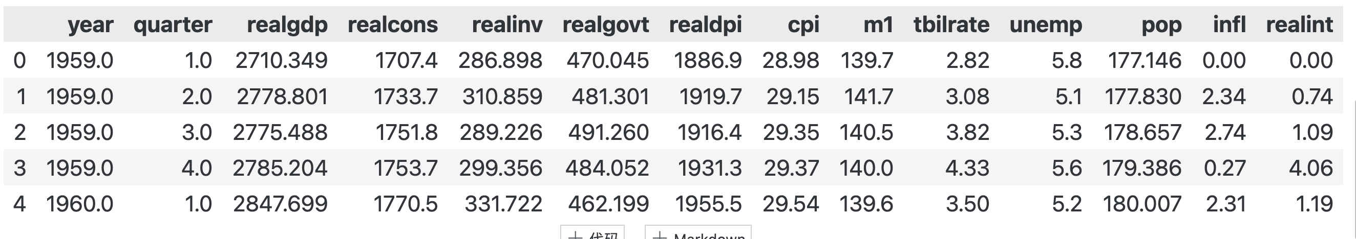
data.info()
data.head()结果:
RangeIndex: 203 entries, 0 to 202
Data columns (total 14 columns):
 #   Column    Non-Null Count  Dtype
---  ------    --------------  -----
 0   year      203 non-null    float64
 1   quarter   203 non-null    float64
 2   realgdp   203 non-null    float64
 3   realcons  203 non-null    float64
 4   realinv   203 non-null    float64
 5   realgovt  203 non-null    float64
 6   realdpi   203 non-null    float64
 7   cpi       203 non-null    float64
 8   m1        203 non-null    float64
 9   tbilrate  203 non-null    float64
 10  unemp     203 non-null    float64
 11  pop       203 non-null    float64
 12  infl      203 non-null    float64
 13  realint   203 non-null    float64
dtypes: float64(14)
memory usage: 22.3 KB
数据格式:
二、Data Prep 数据处理
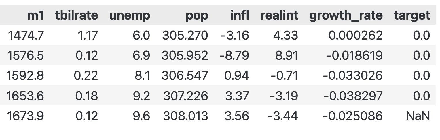
为了获得一个二元目标变量,我们计算季度实际GDP年增长率的20个季度滚动平均值。然后,如果当前增长超过移动平均值,我们将其分配为1,否则分配为0。最后,我们移动指标变量,使下一季度的结果与当前季度对齐。
To obtain a binary target variable, we compute the 20-quarter rolling average of the annual growth rate of quarterly real GDP. We then assign 1 if current growth exceeds the moving average and 0 otherwise. Finally, we shift the indicator variables to align next quarter's outcome with the current quarter.
data['growth_rate'] = data.realgdp.pct_change(4)
data['target'] = (data.growth_rate > data.growth_rate.rolling(20).mean()).astype(int).shift(-1)
data.quarter = data.quarter.astype(int)
data.target.value_counts()
data.tail()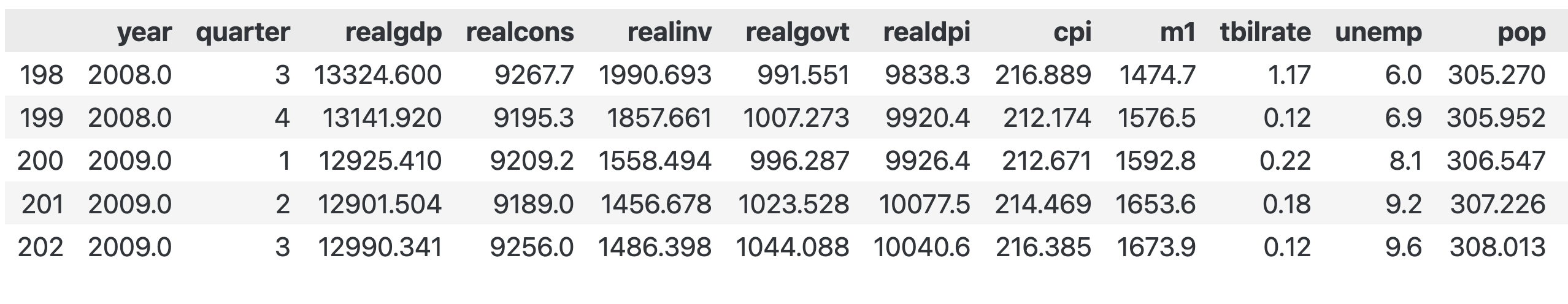
pct_cols = ['realcons', 'realinv', 'realgovt', 'realdpi', 'm1']
drop_cols = ['year', 'realgdp', 'pop', 'cpi', 'growth_rate']
data.loc[:, pct_cols] = data.loc[:, pct_cols].pct_change(4)
data = pd.get_dummies(data.drop(drop_cols, axis=1), columns=['quarter'], drop_first=True).dropna()
data.info()
data.head()
Index: 198 entries, 4 to 201
Data columns (total 13 columns):
 #   Column     Non-Null Count  Dtype
---  ------     --------------  -----
 0   realcons   198 non-null    float64
 1   realinv    198 non-null    float64
 2   realgovt   198 non-null    float64
 3   realdpi    198 non-null    float64
 4   m1         198 non-null    float64
 5   tbilrate   198 non-null    float64
 6   unemp      198 non-null    float64
 7   infl       198 non-null    float64
 8   realint    198 non-null    float64
 9   target     198 non-null    float64
 10  quarter_2  198 non-null    bool
 11  quarter_3  198 non-null    bool
 12  quarter_4  198 non-null    bool
dtypes: bool(3), float64(10)
memory usage: 17.6 KB 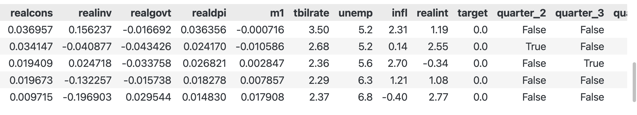
三、Fit Model 拟合模型
# model = sm.Logit(data.target, sm.add_constant(data.drop('target', axis=1)))  # bad code
model = sm.Logit(data.target, sm.add_constant(data.drop('target', axis=1).astype(float)))
result = model.fit()
result.summary()注意,原作者代码已经失效,要加上数据转换才行:
# model = sm.Logit(data.target, sm.add_constant(data.drop('target', axis=1))) # bad code
model = sm.Logit(data.target, sm.add_constant(data.drop('target', axis=1).astype(float)))
结果:
Optimization terminated successfully. Current function value: 0.342965 Iterations 8
| Dep. Variable: | target | No. Observations: | 198 |
|---|---|---|---|
| Model: | Logit | Df Residuals: | 185 |
| Method: | MLE | Df Model: | 12 |
| Date: | Wed, 01 Oct 2025 | Pseudo R-squ.: | 0.5022 |
| Time: | 11:27:45 | Log-Likelihood: | -67.907 |
| converged: | True | LL-Null: | -136.42 |
| Covariance Type: | nonrobust | LLR p-value: | 2.375e-23 |
| coef | std err | z | P>|z| | [0.025 | 0.975] | |
|---|---|---|---|---|---|---|
| const | -8.5881 | 1.908 | -4.502 | 0.000 | -12.327 | -4.849 |
| realcons | 130.1446 | 26.633 | 4.887 | 0.000 | 77.945 | 182.344 |
| realinv | 18.8414 | 4.053 | 4.648 | 0.000 | 10.897 | 26.786 |
| realgovt | -19.0318 | 6.010 | -3.166 | 0.002 | -30.812 | -7.252 |
| realdpi | -52.2473 | 19.912 | -2.624 | 0.009 | -91.275 | -13.220 |
| m1 | -1.3462 | 6.177 | -0.218 | 0.827 | -13.453 | 10.761 |
| tbilrate | 60.8607 | 44.350 | 1.372 | 0.170 | -26.063 | 147.784 |
| unemp | 0.9487 | 0.249 | 3.818 | 0.000 | 0.462 | 1.436 |
| infl | -60.9647 | 44.362 | -1.374 | 0.169 | -147.913 | 25.984 |
| realint | -61.0453 | 44.359 | -1.376 | 0.169 | -147.987 | 25.896 |
| quarter_2 | 0.1128 | 0.618 | 0.182 | 0.855 | -1.099 | 1.325 |
| quarter_3 | -0.1991 | 0.609 | -0.327 | 0.744 | -1.393 | 0.995 |
| quarter_4 | 0.0007 | 0.608 | 0.001 | 0.999 | -1.191 | 1.192 |
四、Analyze 结果分析
McFadden Pseudo R² = 0.50, 模型效果还不错。
我们使用截距并将季度值转换为虚拟变量,并按照以下方式训练逻辑回归模型:
这为我们的模型生成了以下摘要,该模型有198个观测值和13个变量(注:12个变量+截距=13),包括截距:
摘要表明,该模型已使用最大似然法进行训练,并提供对数似然函数在-67.9处的最大值。
We use an intercept and convert the quarter values to dummy variables and train the logistic regression model as follows:
This produces the following summary for our model with 198 observations and 13 variables, including intercept: The summary indicates that the model has been trained using maximum likelihood and provides the maximized value of the log-likelihood function at -67.9.
plt.rc('figure', figsize=(12, 7))
plt.text(0.01, 0.05, str(result.summary()), {'fontsize': 14}, fontproperties = 'monospace')
plt.axis('off')
plt.tight_layout()
plt.subplots_adjust(left=0.2, right=0.8, top=0.8, bottom=0.1)
plt.savefig('logistic_example.png', bbox_inches='tight', dpi=300);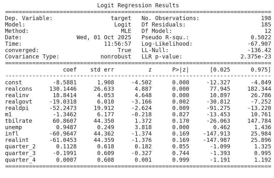


 浙公网安备 33010602011771号