latex 长表格,多子图
##
Journal abbreviation: https://blog.csdn.net/zseqsc_asd/article/details/96895773
\usepackage{cite} %合并多个引用参考文献的数字 [5]-[8]
## 图片部分
\begin{figure}[htbp]%[!t]%[H]%[!h]% [htbp]
\centering
\vspace{-0.35cm} %设置与上面正文的距离
\subfigtopskip=2pt %设置子图与上面正文或别的内容的距离
\subfigbottomskip=2pt %设置第二行子图与第一行子图的距离,即下面的头与上面的脚的距离
\subfigcapskip=-5pt %设置子图与子标题之间的距离
\begin{minipage}[b]{0.33\textwidth}
\includegraphics[width=\textwidth]{final_legend} \\
\end{minipage}
\\ \vspace{-4mm}
\subfigure[]{
\centering \includegraphics[width=0.23\linewidth, keepaspectratio=false]{4_models_Q_airfoil.eps}
}%\hspace{-10pt}
\subfigure[]{
\centering \includegraphics[width=0.23\linewidth, keepaspectratio=false]{4_models_Q_abalone.eps}
}%\hspace{-10pt}
\subfigure[]{
\centering \includegraphics[width=0.23\linewidth, keepaspectratio=false]{4_models_Q_qsar.eps}
}%\hspace{-10pt}
\subfigure[]{
\centering \includegraphics[width=0.23\linewidth, keepaspectratio=false]{4_models_Q_concrete.eps}
}%\hspace{-10pt}
\
\subfigure[]{
\centering \includegraphics[width=0.23\linewidth, keepaspectratio=false]{4_models_Q_pm10.eps}
}%\hspace{-10pt}
\subfigure[]{
\centering \includegraphics[width=0.23\linewidth, keepaspectratio=false]{4_models_Q_housing.eps}
}%\hspace{-10pt}
\subfigure[]{
\centering \includegraphics[width=0.23\linewidth, keepaspectratio=false]{4_models_Q_stock.eps}
}%\hspace{-10pt}
\subfigure[]{
\centering \includegraphics[width=0.23\linewidth, keepaspectratio=false]{4_models_Q_delta.eps}
}%\hspace{-10pt}
\
\subfigure[]{
\centering \includegraphics[width=0.23\linewidth, keepaspectratio=false]{4_models_Q_redwine.eps}
}%\hspace{-10pt}
\subfigure[]{
\centering \includegraphics[width=0.23\linewidth, keepaspectratio=false]{4_models_Q_ccpp.eps}
}
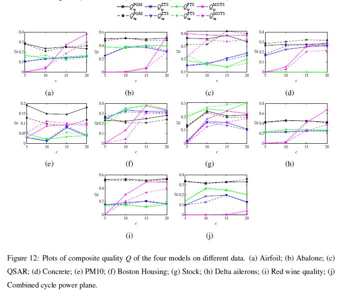
\caption{Plots of composite quality \(Q\) of the four models on different data. (a) Airfoil; (b) Abalone; (c) QSAR; (d) Concrete; (e) PM10; (f) Boston Housing; (g) Stock; (h) Delta ailerons; (i) Red wine quality; (j) Combined cycle power plane.}\label{Fig:AllDatasets_Q_comp}
\end{figure}
点击查看代码
%对表格中Line进行粗细和着色
\usepackage{booktabs}%粗心,可用用toprule,midrule bottomrul
\usepackage{colortbl} %arrayrulecolor{red}hline 可以使得线变为红色
\usepackage{enumerate}%自定义排列顺序
% Some very useful LaTeX packages include:
% (uncomment the ones you want to load)
\usepackage{array}
\usepackage{longtable,booktabs} % 长表格自动分页,此宏包依赖array宏包
\usepackage{multirow} %不规则表格占用多行
%给表格添加注释
\usepackage{threeparttable}
\usepackage{makecell}%表格强行换行
\begin{table}[H]
\centering
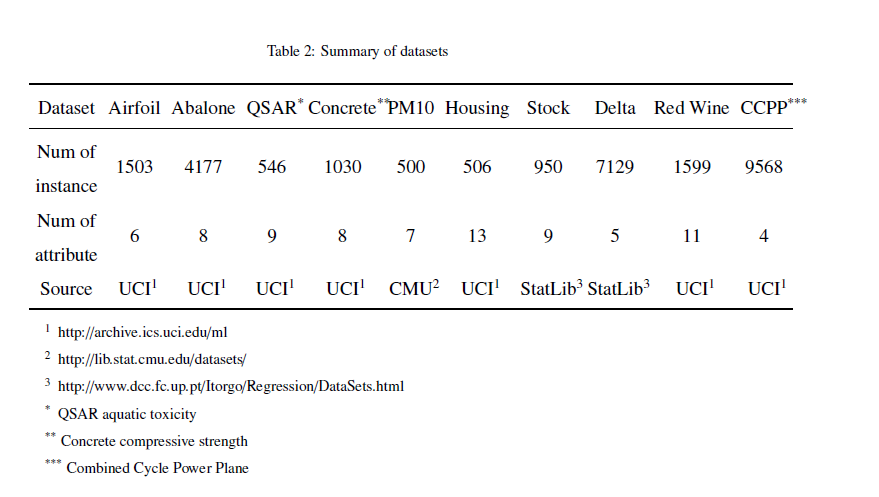
\caption{Summary of datasets}\label{Tab:datasets_summary}
\setlength{\tabcolsep}{1mm}%{XXXX}
%\tiny
\begin{threeparttable}
\begin{tabular}{ccccccccccc}
%\hline
% after \\: \hline or \cline{col1-col2} \cline{col3-col4} ...
%\\
%\hline
\toprule
Dataset &Airfoil & Abalone &QSAR\tnote{*} &Concrete\tnote{**} &PM10& Housing&Stock &Delta&Red Wine&CCPP\tnote{***} \\
\midrule
\makecell[c]{Num of \\ instance}&1503&4177&546&1030&500&506&950&7129&1599&9568\\
\makecell[c]{Num of \\ attribute}&6 &8 &9 &8 &7 &13 &9 &5 &11 &4 \\
Source &UCI\tnote{1}&UCI\tnote{1}&UCI\tnote{1}&UCI\tnote{1}&CMU\tnote{2}&UCI\tnote{1}&StatLib\tnote{3}&StatLib\tnote{3}&UCI\tnote{1}&UCI\tnote{1}\\
\bottomrule
\end{tabular}
\begin{tablenotes}
\footnotesize
\item[1] http://archive.ics.uci.edu/ml
\item[2] http://lib.stat.cmu.edu/datasets/
\item[3] http://www.dcc.fc.up.pt/Itorgo/Regression/DataSets.html
\item[*] QSAR aquatic toxicity
\item[**] Concrete compressive strength
\item[***] Combined Cycle Power Plane
\end{tablenotes}
\end{threeparttable}
\end{table}
\begin{figure}[htb]
\centering
\vspace{-0.35cm} %设置与上面正文的距离
\subfigtopskip=2pt %设置子图与上面正文或别的内容的距离
\subfigbottomskip=2pt %设置第二行子图与第一行子图的距离,即下面的头与上面的脚的距离
\subfigcapskip=-5pt %设置子图与子标题之间的距离
\subfigure[]{
\begin{minipage}[b]{0.3\textwidth}
\includegraphics[width=\textwidth]{D2_inf_grans_inputspace_beta0.eps} \\
\includegraphics[width=\textwidth]{D2_inf_grans_inputoutputspace_beta0.eps}
\end{minipage}
}\hspace{-4mm}
\subfigure[]{
\begin{minipage}[b]{0.3\textwidth}
\includegraphics[width=\textwidth]{D2_inf_grans_inputspace_beta4.eps} \\
\includegraphics[width=\textwidth]{D2_inf_grans_inputoutputspace_beta4.eps}
\end{minipage}
}\hspace{-4mm}
\subfigure[]{
\begin{minipage}[b]{0.3\textwidth}
\includegraphics[width=\textwidth]{D2_inf_grans_inputspace_beta20.eps} \\
\includegraphics[width=\textwidth]{D2_inf_grans_inputoutputspace_beta20.eps}
\end{minipage}
}
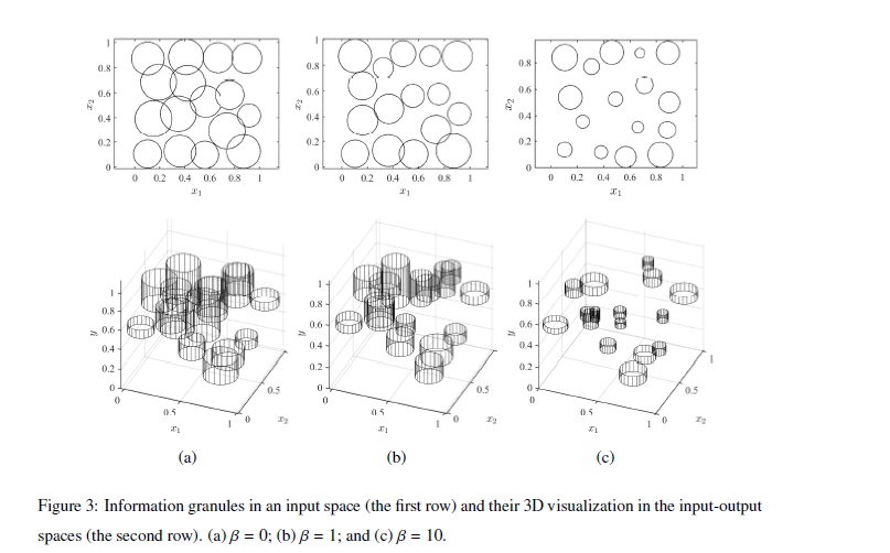
\caption{Information granules in an input space (the first row) and their 3D visualization in the input-output spaces (the second row). (a) \(\beta=0\); (b) \(\beta=1\); and (c) \(\beta=10\).}\label{Fig:beta_impacts_infor_grans}
\end{figure}
##表格部分
###所用宏包
\usepackage{array}
\usepackage{longtable} % 长表格自动分页,此宏包依赖array宏包
\usepackage{multirow} %不规则表格占用多行
\usepackage{makecell} % 强制换行表格 \makecell[居中情况]{第1行内容 \\ 第2行内容 \\ 第3行内容 ...}
合并表格
\begin{table}[h!]
  \centering
  \caption{Comparative results of coverage and specificity for synthetic 1-D numeric data with six clusters for selected values of $c$}\label{Tab:comp_TS_Granular_M}
  \begin{tabular}{ccccccccc}
    %\hline
  \setlength{\tabcolsep}{1mm}%{XXXX} %指定小表格的宽度
    % after \\: \hline or \cline{col1-col2} \cline{col3-col4} ...
     %\\
    %\hline
    \toprule
    \multirow{3}{*}{$c$} &\multicolumn{4}{c}{Standard granular TS model}             &   \multicolumn{4}{c}{Proposed granular fuzzy model} \\
                       \cline{2-9}
                        &\multicolumn{2}{c}{Coverage} &\multicolumn{2}{c}{Specificity} &\multicolumn{2}{c}{Coverage} &\multicolumn{2}{c}{Specificity} \\
                        \cline{2-9}
                        & Training& Testing& Training& Testing                   & Training& Testing& Training& Testing\\
    \midrule
    2                  &0.5976   &0.5111   &0.4996  &0.4391                      &0.1667   & 0.1611 &0.1579  &0.1504\\
    3                  &0.5952   &0.5889   &0.5188  &0.4970                      &0.2429   & 0.1444 &0.2133  &0.1242 \\
    4                  &0.7214   &0.7667   &0.6374  &0.6161                      &0.4738   & 0.4889 &0.4412  &0.4533 \\
    6                  &0.7000   &0.7056   &0.6622  &0.6704                      &0.6786   & 0.6556 &0.6403  &0.6172  \\
    8                  &0.6167   &0.5556   &0.5907  &0.5357                      &0.8000   & 0.8000 &0.7324  &0.7386  \\
    10                 &0.5524   &0.5167   &0.5336  &0.5029                      &0.8289   & 0.8167 &0.7707  &0.7673  \\
    %12                 &0.9357   &0.9389   &0.8751  &0.8791                      &0.8190   & 0.9000 &0.7519  &0.8273  \\
\bottomrule

\end{tabular}
\end{table}

###长算法表格,跨页显示
\begin{longtable}{p{\linewidth}}
\toprule
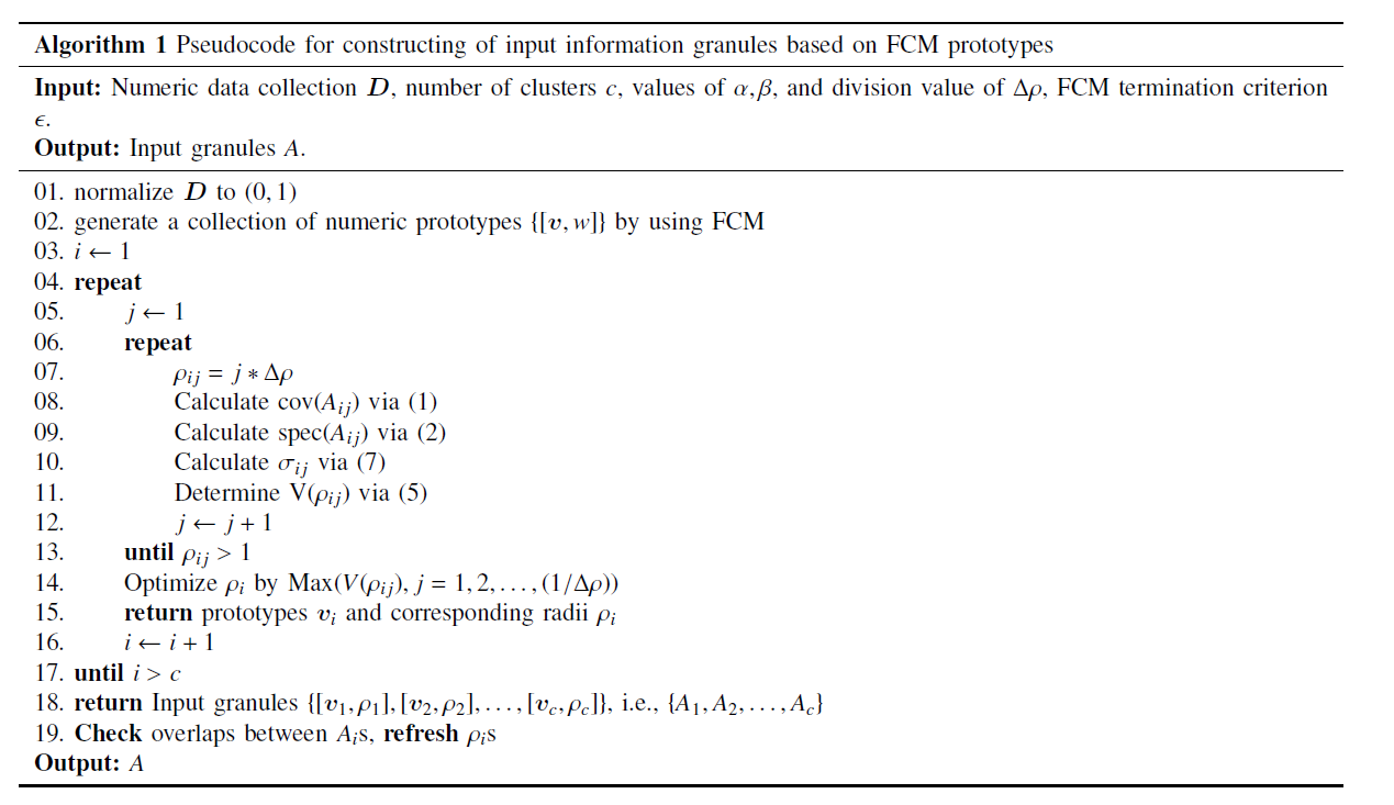
\textbf{Algorithm 1} Pseudocode for constructing of input information granules based on FCM prototypes \\
\endfirsthead
% Appear the table header at the top of every page
\toprule
\textbf{Algorithm 1} Pseudocode for constructing of input information granules based on FCM prototypes \
\hline
\endhead
% Appear \hline at the bottom of every page
\hline
\endfoot
\midrule
\textbf{Input:} Numeric data collection \(\bm D\), number of clusters \(c\), values of \(\alpha, \beta\), and division value of \(\Delta \rho\), FCM termination criterion \(\epsilon\).\
\textbf{Output:} Input granules \(A\). \
\midrule
- normalize \(\bm D\) to \((0,1)\) \
- generate a collection of numeric prototypes \(\{ [\bm v, w]\}\) by using FCM \
- \(i\leftarrow 1\) \
- \textbf{repeat} \
-
\qquad $j\leftarrow1$\\
-
\qquad \textbf{repeat}\\
-
\qquad\qquad $\rho_{ij} = j*\Delta\rho$\\
-
\qquad\qquad Calculate ${\rm cov}(A_{ij})$ via \eqref{Eq:cov} \\
-
\qquad\qquad Calculate ${\rm spec}(A_{ij})$ via \eqref{Eq:spec} \\
-
\qquad\qquad Calculate $\sigma_{ij}$ via \eqref{Eq:diviation_y}\\
-
\qquad\qquad Determine V($\rho_{ij}$) via \eqref{Eq:input_gran_radus_value} \\
-
\qquad\qquad $j\leftarrow j+1$\\
-
\qquad \textbf{until} $\rho_{ij}>1$\\
-
\qquad Optimize $\rho_{i}$ by Max$( V(\rho_{ij}), j=1,2,\ldots,(1/\Delta\rho) )$\\
-
\qquad \textbf{return} prototypes $\bm v_{i}$ and corresponding radii $\rho_{i}$\\
-
\qquad $i \leftarrow i+1$\\
- \textbf{until} \(i>c\)\
- \textbf{return} Input granules \(\{ [\boldsymbol v_{1},\rho_{1}], [\boldsymbol v_{2},\rho_{2}],\ldots,[\boldsymbol v_{c},\rho_{c}] \}\), i.e., \(\{ A_{1},A_{2},\ldots,A_{c} \}\)\
- \textbf{Check} overlaps between \(A_{i}\)s, \textbf{refresh} \(\rho_{i}\)s \
\noindent \textbf{Output:} \(A\) \
\bottomrule
\end{longtable}
### 表格添加注释
https://www.jianshu.com/p/110714b2a535
### LATEX使用subfigure命令插入多行多列图片并且为子图模式 修改子图与子图、子标题的距离
###latex 插入图片将Figure 改为Fig.
https://blog.csdn.net/ynpeng531/article/details/96450217
### LaTeX表格内部,强行换行
https://www.jianshu.com/p/b6b45402d8b2
###作者信息不能挨着
第一步:
打开IEEEtran.cls(建议使用notepad打开,比较规整)
第二步:
找到\def\@IEEEBIOskipN{4\baselineskip}% nominal value of the vskip above the biography
然后将4改为1,即可。
https://blog.csdn.net/qq_29086043/java/article/details/89243190
参考文献更改 杂志名称缩写
https://www.cnblogs.com/tsingke/p/4523908.html
##公式部分
\sum \nolimits_{k} 是下标 
在文本正上方加入符号,用这个命令\mathop {y(x)}\limits^{\ast}
Z 正下方 \mathop {H}\limits_{1}
##bib文件路径设置
如何能只维护一个bib文件,而使多个tex文档都能引用到它?折腾了两个小时搞定了。百度翻了好几页都没有解决,还是google用英文搜索找到的。看来以后不能偷懒总找中文资料。记下来以备需要的人能中文搜索到。
总结下来有两个解决办法,一个是绝对路径引用,一个是相对路径引用。
绝对路径引用在末尾用\bibliography{E:/.../bibliography} 此处注意用/而不用\. 另外路径过程中不能有空格。例如其中有一级文件夹名字叫latex study就不行,得改成latex_study才可以。
相对路径引用,在导言区重新定义路径。举例如下:
documentclass{<class>}
\newcommand{\myreferences}{../references/bibliography}
%...
\begin{document}
%...
\bibliography{\myreferences}
%...
\end{document}
此处同样注意,路径中各级文件夹名字都不能有空格,否则latex找不到,引用处会出现问号。切记切记。
这是我看下来比较容易的办法,其他的方法需要根据编辑器或者操作系统作修改,比较复杂
出处http://blog.sina.com.cn/s/blog_88e43f760102v585.html

 浙公网安备 33010602011771号