

大数据分析第三周作业
import pandas as pd
datafile='D:\zy3\\air_data.csv'
resultfile='D:\zy3\\explore.csv'
data = pd.read_csv(datafile,encoding = 'utf-8')
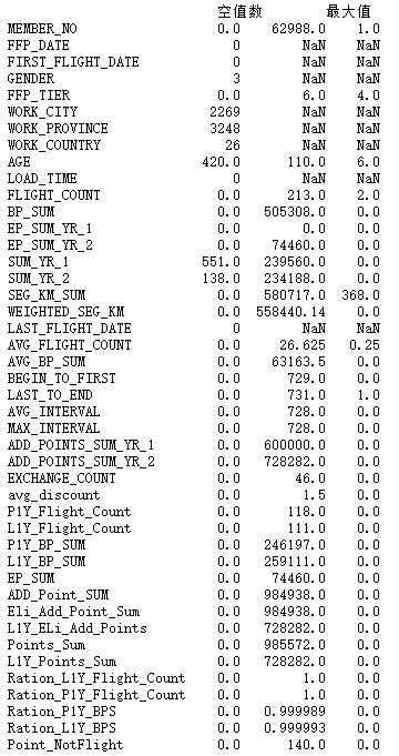
explore = data.describe(percentiles = [],include = 'all').T
explore['null'] = len(data)-explore['count']
explore = explore[['null','max','min']]
explore.columns = [u'空值数',u'最大值',u'最小值']
explore.to_csv(resultfile)
print(explore)
from datetime import datetime
import matplotlib.pyplot as plt
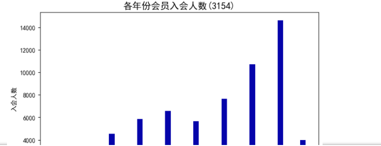
ffp=data['FFP_DATE'].apply(lambda x:datetime.strptime(x,'%Y/%m/%d'))
ffp_year=ffp.map(lambda x:x.year)
#绘制各年份会员入会人数直方图
fig=plt.figure(figsize=(8,5))
plt.rcParams['font.sans-serif']='SimHei'
plt.rcParams['axes.unicode_minus']='False'
plt.hist(ffp_year,bins='auto',color='#0504aa')
plt.xlabel('年份')
plt.ylabel('入会人数')
plt.title('各年份会员入会人数(3154)',fontsize=15)
plt.show()
plt.close
#提取会员不同性别人数
male=pd.value_counts(data['GENDER'])['男']
female=pd.value_counts(data['GENDER'])['女']
#绘制会员性别比例饼图
fig=plt.figure(figsize=(10,6))
plt.pie([male,female],labels=['男','女'],colors=['lightskyblue','lightcoral'],autopct='%1.1f%%')
plt.title('会员性别比例(3135)',fontsize=15)
plt.show()
plt.close()
#提取不同级别会员人数
lv_four=pd.value_counts(data['FFP_TIER'])[4]
lv_five=pd.value_counts(data['FFP_TIER'])[5]
lv_six=pd.value_counts(data['FFP_TIER'])[6]
#绘制会员各级别人数条形图
fig=plt.figure(figsize=(8,5))
plt.bar(x=range(3),height=[lv_four,lv_five,lv_six],width=0.4,alpha=0.8,color='skyblue')
plt.xticks([index for index in range(3)],['4','5','6'])
plt.xlabel('会员等级')
plt.ylabel('会员人数')
plt.title('会员各级别人数(3154)',fontsize=15)
plt.show()
plt.close
#提取会员年龄
age=data['AGE'].dropna()
age=age.astype('int64')
#绘制会员年龄分布箱型图
fig=plt.figure(figsize=(5,10))
plt.boxplot(age,
patch_artist=True,
labels=['会员年龄'],
boxprops={'facecolor':'lightblue'})
plt.title('会员年龄分布箱型图(3154)',fontsize=15)
plt.grid(axis='y')
plt.show()
plt.close()
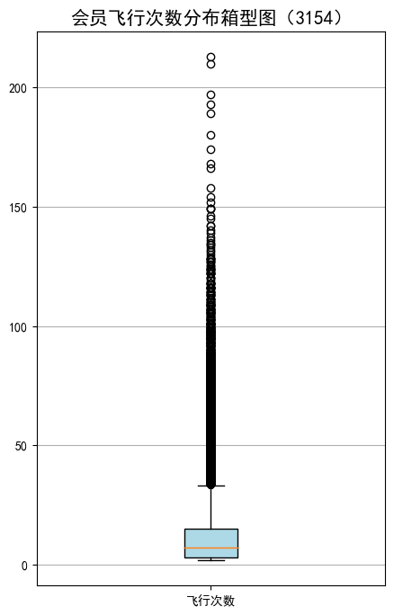
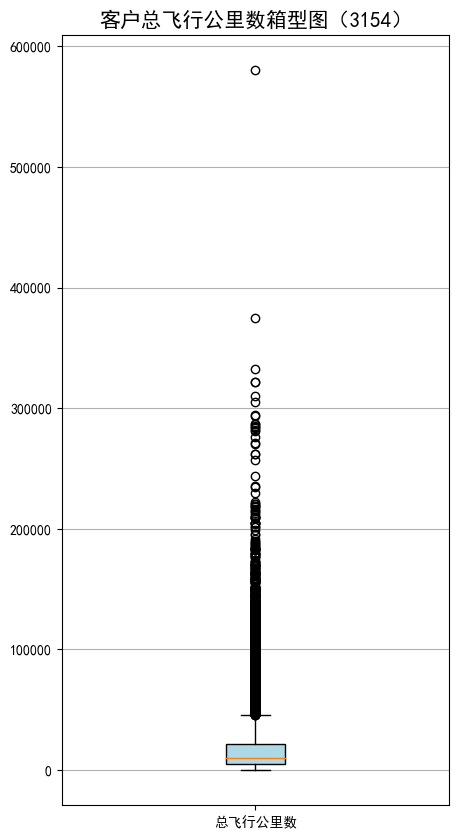
lte=data['LAST_TO_END']
fc=data['FLIGHT_COUNT']
sks=data['SEG_KM_SUM']
#绘制最后乘机至结束时长箱型图
fig=plt.figure(figsize=(5,8))
plt.boxplot(lte,
patch_artist=True,
labels=['时长'],
boxprops={'facecolor':'lightblue'})
plt.title('会员最后乘机至结束时长分布箱型图(3154)',fontsize=15)
plt.grid(axis='y')
plt.show()
plt.close
#绘制客户飞行次数箱型图
fig=plt.figure(figsize=(5,8))
plt.boxplot(fc,
patch_artist=True,
labels=['飞行次数'],
boxprops={'facecolor':'lightblue'})
plt.title('会员飞行次数分布箱型图(3154)',fontsize=15)
plt.grid(axis='y')
plt.show()
plt.close
#绘制客户总飞行公里数箱型图
fig=plt.figure(figsize=(5,10))
plt.boxplot(sks,
patch_artist=True,
labels=['总飞行公里数'],
boxprops={'facecolor':'lightblue'})
plt.title('客户总飞行公里数箱型图(3154)',fontsize=15)
plt.grid(axis='y')
plt.show()
plt.close
#积分信息类别
#提取会员积分兑换次数
ec=data['EXCHANGE_COUNT']
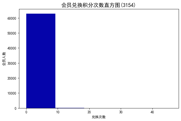
#绘制会员兑换积分次数直方图
fig=plt.figure(figsize=(8,5))
plt.hist(ec,bins=5,color='#0504aa')
plt.xlabel('兑换次数')
plt.ylabel('会员人数')
plt.title('会员兑换积分次数直方图(3154)',fontsize=15)
plt.show()
plt.close
#提取会员总累计积分
ps=data['Points_Sum']
#绘制会员总累计积分箱型图
fig=plt.figure(figsize=(5,8))
plt.boxplot(ps,
patch_artist=True,
labels=['总累计积分'],
boxprops={'facecolor':'lightblue'})
plt.title('客户总累计积分箱型图(3154)',fontsize=15)
plt.grid(axis='y')
plt.show()
plt.close

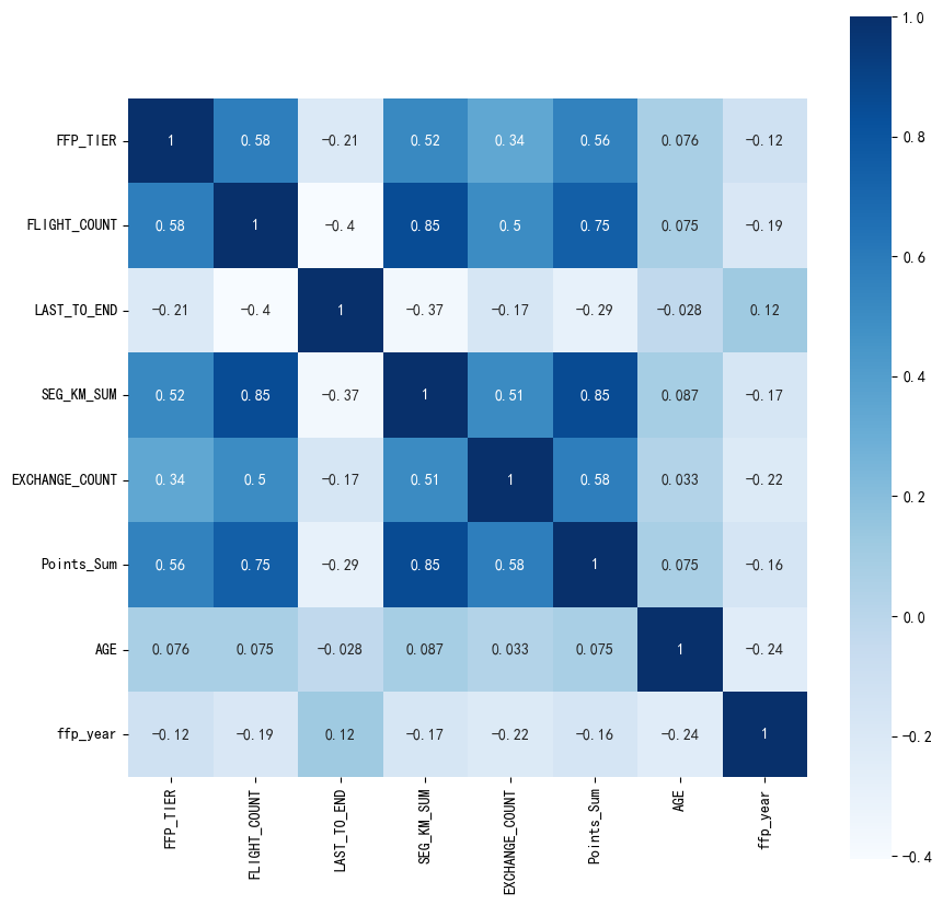
#提取属性并合并为新数据集
data_corr=data[['FFP_TIER','FLIGHT_COUNT','LAST_TO_END','SEG_KM_SUM','EXCHANGE_COUNT','Points_Sum']]
age1=data['AGE'].fillna(0)
data_corr['AGE']=age1.astype('int64')
data_corr['ffp_year']=ffp_year
#计算相关性矩阵
dt_corr=data_corr.corr(method='pearson')
print('相关性矩阵为:\n',dt_corr)
#绘制热力图
import seaborn as sns
plt.subplots(figsize=(10,10))
sns.heatmap(dt_corr,annot=True,vmax=1,square=True,cmap='Blues')
plt.show()
plt.close
相关性矩阵为:
                 FFP_TIER  FLIGHT_COUNT  LAST_TO_END  SEG_KM_SUM  \
FFP_TIER        1.000000      0.582447    -0.206313    0.522350
FLIGHT_COUNT    0.582447      1.000000    -0.404999    0.850411
LAST_TO_END    -0.206313     -0.404999     1.000000   -0.369509
SEG_KM_SUM      0.522350      0.850411    -0.369509    1.000000
EXCHANGE_COUNT  0.342355      0.502501    -0.169717    0.507819
Points_Sum      0.559249      0.747092    -0.292027    0.853014
AGE             0.076245      0.075309    -0.027654    0.087285
ffp_year       -0.116510     -0.188181     0.117913   -0.171508

                EXCHANGE_COUNT  Points_Sum       AGE  ffp_year
FFP_TIER              0.342355    0.559249  0.076245 -0.116510
FLIGHT_COUNT          0.502501    0.747092  0.075309 -0.188181
LAST_TO_END          -0.169717   -0.292027 -0.027654  0.117913
SEG_KM_SUM            0.507819    0.853014  0.087285 -0.171508
EXCHANGE_COUNT        1.000000    0.578581  0.032760 -0.216610
Points_Sum            0.578581    1.000000  0.074887 -0.163431
AGE                   0.032760    0.074887  1.000000 -0.242579
ffp_year             -0.216610   -0.163431 -0.242579  1.000000
import numpy as np
import pandas as pd
datafile ='D:\zy3\\air_data.csv'
cleanedfile='D:\zy3\\data_cleaned.csv'
#读取数据
airline_data=pd.read_csv(datafile,encoding='utf-8')
print('原始数据的形状为:',airline_data.shape)
#去除票价为空的记录
airline_notnull=airline_data.loc[airline_data['SUM_YR_1'].notnull()&airline_data['SUM_YR_2'].notnull(),:]
print('删除缺失记录后数据的形状为:',airline_notnull.shape)
#只保留票价非零的,或者平均折扣率不为0且总飞行公里数大于0的记录
index1=airline_notnull['SUM_YR_1']!=0
index2=airline_notnull['SUM_YR_2']!=0
index3=(airline_notnull['SEG_KM_SUM']>0)&(airline_notnull['avg_discount']!=0)
index4=airline_notnull['AGE']>100#去除年龄大于100的记录
airline=airline_notnull[(index1|index2)&index3&~index4]
print('数据清洗后数据的形状为:',airline.shape)
airline.to_csv(cleanedfile)
原始数据的形状为: (62988, 44)
删除缺失记录后数据的形状为: (62299, 44)
数据清洗后数据的形状为: (62043, 44)
import pandas as pd
import numpy as np
#读取数据清洗后的数据
cleanedfile='D:\zy3\\data_cleaned.csv'
airline=pd.read_csv(cleanedfile,encoding='utf-8')
#选取需求属性
airline_selection=airline[['FFP_DATE','LOAD_TIME','LAST_TO_END','FLIGHT_COUNT','SEG_KM_SUM','avg_discount']]
print('筛选的属性前5行为:\n',airline_selection.head())
筛选的属性前5行为:
     FFP_DATE  LOAD_TIME  LAST_TO_END  FLIGHT_COUNT  SEG_KM_SUM  avg_discount
0  2006/11/2  2014/3/31            1           210      580717      0.961639
1  2007/2/19  2014/3/31            7           140      293678      1.252314
2   2007/2/1  2014/3/31           11           135      283712      1.254676
3  2008/8/22  2014/3/31           97            23      281336      1.090870
4  2009/4/10  2014/3/31            5           152      309928      0.970658
#构造属性L
L=pd.to_datetime(airline_selection['LOAD_TIME']) - \
pd.to_datetime(airline_selection['FFP_DATE'])
L=L.astype('str').str.split().str[0]
L=L.astype('int')/30
#合并属性
airline_features=pd.concat([L,airline_selection.iloc[:,2:]],axis=1)
print('构建的LRFMC属性前5行为:\n',airline_features.head())
#数据标准化
from sklearn.preprocessing import StandardScaler
data=StandardScaler().fit_transform(airline_features)
np.savez('D:\zy3\\airline_scale.npz',data)
print('标准化后LRFMC 5个属性为:\n',data[:5,:])
构建的LRFMC属性前5行为:
            0  LAST_TO_END  FLIGHT_COUNT  SEG_KM_SUM  avg_discount
0  90.200000            1           210      580717      0.961639
1  86.566667            7           140      293678      1.252314
2  87.166667           11           135      283712      1.254676
3  68.233333           97            23      281336      1.090870
4  60.533333            5           152      309928      0.970658
标准化后LRFMC 5个属性为:
 [[ 1.43579256 -0.94493902 14.03402401 26.76115699  1.29554188]
 [ 1.30723219 -0.91188564  9.07321595 13.12686436  2.86817777]
 [ 1.32846234 -0.88985006  8.71887252 12.65348144  2.88095186]
 [ 0.65853304 -0.41608504  0.78157962 12.54062193  1.99471546]
 [ 0.3860794  -0.92290343  9.92364019 13.89873597  1.34433641]]
#K-Means聚类标准化后的数据
import pandas as pd
import numpy as np
from sklearn.cluster import KMeans
#读取标准化后的数据
airline_scale=np.load('D:\zy3\\airline_scale.npz')['arr_0']
k=5 #确定聚类中心
#构建模型,随机种子设为123
kmeans_model=KMeans(n_clusters=k,random_state=123)
fit_kmeans=kmeans_model.fit(airline_scale) #模型训练
#查看聚类结果
kmeans_cc=kmeans_model.cluster_centers_#聚类中心
print('各类聚类中心为:\n',kmeans_cc)
kmeans_labels=kmeans_model.labels_#样本的类别标签
print('各样本的类别标签为:\n',kmeans_labels)
r1=pd.Series(kmeans_model.labels_).value_counts()#统计不同类别样本的数目
print('最终每个类别的数目为:\n',r1)
#输出聚类分群的结果
cluster_center=pd.DataFrame(kmeans_model.cluster_centers_,\
columns=['ZL','ZR','ZF','ZM','ZC'])#将聚类中心放在数据框中
cluster_center.index=pd.DataFrame(kmeans_model.labels_ ).\
drop_duplicates().iloc[:,0]
print(cluster_center)
各类聚类中心为:
 [[-0.70030628 -0.41502288 -0.16081841 -0.16053724 -0.25728596]
 [ 0.0444681  -0.00249102 -0.23046649 -0.23492871  2.17528742]
 [ 0.48370858 -0.79939042  2.48317171  2.42445742  0.30923962]
 [ 1.1608298  -0.37751261 -0.08668008 -0.09460809 -0.15678402]
 [-0.31319365  1.68685465 -0.57392007 -0.5367502  -0.17484815]]
各样本的类别标签为:
 [2 2 2 ... 0 4 4]
最终每个类别的数目为:
 0    24630
3    15733
4    12117
2     5337
1     4226
dtype: int64
         ZL        ZR        ZF        ZM        ZC
0
2 -0.700306 -0.415023 -0.160818 -0.160537 -0.257286
1  0.044468 -0.002491 -0.230466 -0.234929  2.175287
3  0.483709 -0.799390  2.483172  2.424457  0.309240
0  1.160830 -0.377513 -0.086680 -0.094608 -0.156784
4 -0.313194  1.686855 -0.573920 -0.536750 -0.174848

 浙公网安备 33010602011771号