Tensorflow学习报告

张量

import tensorflow as tf
#创建常量
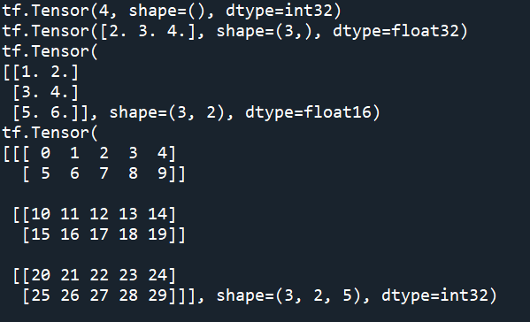
rank_0_tensor = tf.constant(4)   
print(rank_0_tensor)
#创建一阶张量（向量）
rank_1_tensor = tf.constant([2.0, 3.0, 4.0])   
print(rank_1_tensor)
#创建二阶张量（向量）
rank_2_tensor = tf.constant([[1, 2],
                             [3, 4],
                             [5, 6]], dtype=tf.float16)
print(rank_2_tensor)
#创建三阶张量（向量）
rank_3_tensor = tf.constant([
  [[0, 1, 2, 3, 4],
   [5, 6, 7, 8, 9]],
  [[10, 11, 12, 13, 14],
   [15, 16, 17, 18, 19]],
  [[20, 21, 22, 23, 24],
   [25, 26, 27, 28, 29]],])

print(rank_3_tensor)

　　

张亮运算

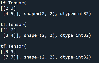
a = tf.constant([[1, 2],
                 [3, 4]])
b = tf.constant([[1, 1],
                 [1, 1]])

print(tf.add(a, b), "\n")  #加法
print(tf.multiply(a, b), "\n")  #逐元素乘法
print(tf.matmul(a, b), "\n")  #矩阵乘法

形状操作

tf.shape([[[1, 1, 1], [2, 2, 2]], [[3, 3, 3], [4, 4, 4]]],name=None)  #返回数据的shape
tf.Tensor([2 2 3], shape=(3,), dtype=int32)

tf.size([[[1, 1, 1], [2, 2, 2]], [[3, 3, 3], [4, 4, 4]]], name=None) #返回数据的元素数量
tf.Tensor(12, shape=(), dtype=int32)
tf.rank([[[1, 1, 1], [2, 2, 2]], [[3, 3, 3], [4, 4, 4]]],name=None) #返回tensor的rank
tf.Tensor(3, shape=(), dtype=int32)

 

低阶API实现线性回归

import tensorflow as tf
import numpy as np
import matplotlib.pyplot as plt
input_x=np.float32(np.linspace(-1,1,100))#在区间[-1,1)内产生100个数的等差数列，作为输入
input_y=2*input_x+np.random.randn(*input_x.shape)*0.3#y=2x+随机噪声
weight=tf.Variable(1.,dtype=tf.float32,name='weight')
bias=tf.Variable(1.,dtype=tf.float32,name='bias')
def model(x):          #定义了线性模型y=weight*x+bias
    pred=tf.multiply(x, weight)+bias
    return pred
step=0
opt=tf.optimizers.Adam(1e-1) #选择优化器，是一种梯度下降的方法
for x,y in zip(input_x,input_y):
    x=np.reshape(x,[1])
    y=np.reshape(y,[1])
    step=step+1
    with tf.GradientTape()as tape:
        loss=tf.losses.MeanSquaredError()(model(x),y)#连续数据的预测，损失函数用MSE
    grads=tape.gradient(loss,[weight,bias])#计算梯度
    opt.apply_gradients(zip(grads,[weight,bias]))#更新参数weight和bias
    print("Step:",step,"Traing Loss:",loss.numpy())
    #用Matplotlib可视化原始数据和预测的模型
    plt.plot(input_x,input_y,'ro',label='original data')
    plt.plot(input_x, model(input_x),label='predicted value')
    plt.plot(input_x,2*input_x,label='y=2x')
    plt.legend()
    plt.show()
    print(weight)
    print(bias)