数据分析框架：实现99%准确率

　　我写这篇文章的目的，是为参加数据科学社区Kaggle简单指引。 大多数初学者无从下手，因为他们使用自己不理解的库和算法，就像陷入黑盒。 本教程将通过提供一个框架来教您如何像数据科学家一样思考与编码，从而为您提供数据分析的领域优势。 

目录：

一 、引言：数据科学家如何打败赔率

二 、 数据科学框架综述

三、步骤1：明确问题、步骤2：准备数据

四、步骤3：数据清洗

五、数据清理的4 C：纠正，完成，创建和转换

六、步骤4：进行探索性分析

七、步骤5：模型数据

八、评估模型性能

九、具有超参数的调整模型

十、具有特征选择的调整模型

十一、步骤6：验证和实施

十二、步骤7：优化和制定战略

---

一 、引言：数据科学家如何打败赔率

　　预测二元事件的结果是一个经典的问题。 例如，你赢了或没赢，你通过测试或没有通过测试。 常见的业务应用程序是流失或客户保留。 另一个流行的用例是医疗保健的死亡率或生存分析。 二进制事件创建了一个有趣的动态，因为我们从统计上知道，随机猜测应该达到50％的准确率，就像投硬币一样，而无需创建单个算法或编写一行代码。 然而，就像自动更正拼写检查技术一样，有时我们人类可能因为自己的利益而过于聪明，实际上表现不如硬币翻转。 在本文中，我使用Kaggle的入门竞赛，泰坦尼克号数据，介绍如何使用数据科学框架来克服困难。

二 、 数据科学框架综述

1. 定义问题：俗话说，不要把车放在马前。在解决问题之前，必须要明白问题是什么，而且可以应用以前的模型或者算法，而不是直接尝试新的方法。
2. 收集数据：约翰·奈斯比特在他1984年的书“大趋势”中写道，我们“淹没在数据中，但仍然需要知识。”所以，数据集已经存在于某个地方，某种格式。可能是外部或内部的，结构化的或非结构化的，静态的或流式的，客观的或主观的等等。俗话说，你不必重新发明轮子，你只需要知道在哪里找到它。在下一步中，我们担心将“脏数据”转换为“清理数据”。
3. 数据清洗：是将“疯狂”数据转换为“可管理”数据的必需过程。数据包括实现用于存储和处理的数据架构，开发用于质量和控制的数据治理标准，数据提取（即ETL和网络抓取）以及用于识别异常，丢失或异常数据点的数据清理。
4. 探索性分析：任何曾经使用过数据的人都知道，垃圾进入，垃​​圾进出（GIGO）。因此，部署描述性和图形化统计信息以查找数据集中的潜在问题，模式，分类，相关性和比较非常重要。此外，数据分类（即定性与定量）对于理解和选择正确的假设检验或数据模型也很重要。
5. 模型数据：与描述性和推论性统计数据一样，数据建模可以汇总数据或预测未来结果。算法是工具而不是魔法棒或银子弹，你必须知道如何为工作选择合适工具的主人。错误的模型最坏的情况下会导致糟糕的表现和错误的结论。
6. 验证和实施数据模型：在根据数据子集训练模型后，是时候测试模型了。这有助于确保不会过度拟合模型或使其特定于所选子集，因为它不能准确地适合同一数据集中的另一个子集。在这一步中，我们确定我们的模型是否适合，概括或不适合我们的数据集。
7. 优化和策略：你在这个过程中重复一遍，让它更好......更强......比以前更快。作为数据科学家，您的策略应该是将开发人员操作和应用程序管道外包，这样您就有更多时间专注于建议和设计。

三、步骤1：明确问题、步骤2：准备数据

步骤1：定义问题
对于这个项目，问题陈述在上述计划中已经给出，开发一种算法来预测泰坦尼克号上乘客的生存结果。

......

项目概要：RMS泰坦尼克号沉没是历史上最臭名昭着的沉船之一。 1912年4月15日，在她的处女航中，泰坦尼克号在与冰山相撞后沉没，在2224名乘客和机组人员中造

成1502人死亡。这场耸人听闻的悲剧震惊了国际社会，并导致了更好的船舶安全规定。

造成海难失事的原因之一是乘客和机组人员没有足够的救生艇。尽管幸存下沉有一些运气因素，但有些人比其他人更容易生存，比如女人，孩子和上流社会。

在这个挑战中，我们要求您完成对哪些人可能存活的分析。特别是，我们要求您运用机器学习工具来预测哪些乘客幸免于悲剧。

练习技巧

• 二进制分类
• Python知识

第2步：收集数据
Kaggle的泰坦尼克号上的测试和训练数据在：灾难中的机器学习

四、步骤3：数据清洗

步骤3：数据清洗

收集了数据之后，必须对数据进行清洗。

3.1导入所需要的包

下面的代码是用Python 3.x编写的。 预先编写和导入一些库来执行必要的任务。 

# This Python 3 environment comes with many helpful analytics libraries installed
# It is defined by the kaggle/python docker image: https://github.com/kaggle/docker-python

#load packages
import sys #access to system parameters https://docs.python.org/3/library/sys.html
print("Python version: {}". format(sys.version))

import pandas as pd #collection of functions for data processing and analysis modeled after R dataframes with SQL like features
print("pandas version: {}". format(pd.__version__))

import matplotlib #collection of functions for scientific and publication-ready visualization
print("matplotlib version: {}". format(matplotlib.__version__))

import numpy as np #foundational package for scientific computing
print("NumPy version: {}". format(np.__version__))

import scipy as sp #collection of functions for scientific computing and advance mathematics
print("SciPy version: {}". format(sp.__version__)) 

import IPython
from IPython import display #pretty printing of dataframes in Jupyter notebook
print("IPython version: {}". format(IPython.__version__)) 

import sklearn #collection of machine learning algorithms
print("scikit-learn version: {}". format(sklearn.__version__))

#misc libraries
import random
import time


#ignore warnings
import warnings
warnings.filterwarnings('ignore')
print('-'*25)

3.11加载数据和建模的库
　　我们将使用流行的scikit-learn库来开发我们的机器学习算法。 在sklearn中，算法称为Estimators并在其自己的类中实现。 对于数据可视化，我们将使用matplotlib和seaborn库。 以下是要加载的常见类。

#导入所需要的包
#Common Model Algorithms
from sklearn import svm, tree, linear_model, neighbors, naive_bayes, ensemble, discriminant_analysis, gaussian_process
from xgboost import XGBClassifier

#Common Model Helpers
from sklearn.preprocessing import OneHotEncoder, LabelEncoder
from sklearn import feature_selection
from sklearn import model_selection
from sklearn import metrics

#Visualization
import matplotlib as mpl
import matplotlib.pyplot as plt
import matplotlib.pylab as pylab
import seaborn as sns
from pandas.tools.plotting import scatter_matrix

#Configure Visualization Defaults
#%matplotlib inline = show plots in Jupyter Notebook browser
%matplotlib inline
mpl.style.use('ggplot')
sns.set_style('white')
pylab.rcParams['figure.figsize'] = 12,8

3.2了解数据类型
　　通过名字了解数据，并了解它的一些信息。它是什么样的（数据类型和值），是什么使得它（独立/特征变量（s）），它的目标是什么（依赖/目标变量）。

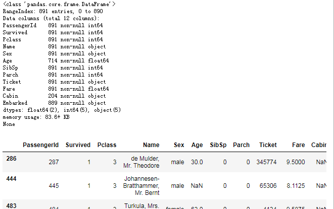
要开始此步骤，我们首先导入数据。接下来，我们使用info（）和sample（）函数来获得可变数据类型（即定性与定量）。单击此处获取源数据。

• 幸存变量（Survived）是我们的结果或因变量。对于幸存者，它是二进制标称数据类型1，而对于死者，它是0。
• PassengerID和Ticket变量假定为随机唯一标识符，对结果变量没有影响。因此，他们将被排除在分析之外。
• Pclass变量是故障单类的序数数据类型，是社会经济阶层（SES）：1 =上层，2 =中产阶级，3 =下层。
• Name变量是标称数据类型。它可以用于特征工程中，从标题中获得性别，从姓氏中获取家庭大小，从医生或主人等标题中获取SES。由于这些变量已经存在，我们将利用它来查看标题，如master，是否有所作为。
• Sex和Embarked变量是名义数据类型。它们将被转换为虚拟变量以进行数学计算。
• Age和Fare变量是连续的定量数据类型。
• SibSp代表船上相关兄弟姐妹/配偶的数量，Parch代表船上相关父母/子女的数量。两者都是离散的定量数据类型。这可以用于特征工程来创建族大小并且是单独变量。
• Cabin变量是一种标称数据类型，可用于特征工程中事件发生时船舶上的大致位置和甲板水平的SES。但是，由于存在许多空值，因此会从分析中排除。

#import data from file: https://pandas.pydata.org/pandas-docs/stable/generated/pandas.read_csv.html
data_raw = pd.read_csv(r'F:\wd.jupyter\datasets\kaggle_data\titanic\train.csv')


#a dataset should be broken into 3 splits: train, test, and (final) validation
#the test file provided is the validation file for competition submission
#we will split the train set into train and test data in future sections
data_val  = pd.read_csv(r'F:\wd.jupyter\datasets\kaggle_data\titanic\test.csv')


#to play with our data we'll create a copy
#remember python assignment or equal passes by reference vs values, 
#so we use the copy function: https://stackoverflow.com/questions/46327494/python-pandas-dataframe-copydeep-false-vs-copydeep-true-vs
data1 = data_raw.copy(deep = True)

#however passing by reference is convenient, because we can clean both datasets at once
data_cleaner = [data1, data_val]


#preview data
print (data_raw.info()) #https://pandas.pydata.org/pandas-docs/stable/generated/pandas.DataFrame.info.html
#data_raw.head() #https://pandas.pydata.org/pandas-docs/stable/generated/pandas.DataFrame.head.html
#data_raw.tail() #https://pandas.pydata.org/pandas-docs/stable/generated/pandas.DataFrame.tail.html
data_raw.sample(10) #https://pandas.pydata.org/pandas-docs/stable/generated/pandas.DataFrame.sample.html

五、数据清理的4 C：纠正，完成，创建和转换

5.1 数据清理的4 C：纠正，完成，创建和转换

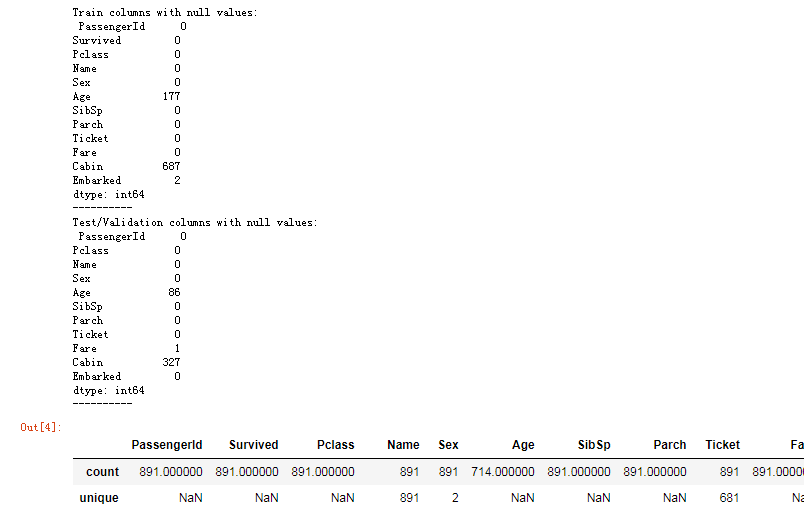
在这个阶段，我们将清理我们的数据：（1）纠正异常值和异常值，（2）完成缺失信息，（3）创建新的分析功能，（4）将字段转换为正确的格式进行计算和显示。

• 更正（correcting）：查看数据时，似乎没有任何异常或不可接受的数据输入。此外，我们发现我们可能在年龄和票价方面存在潜在的异常值。但是，由于它们是合理的值，我们将等到我们完成探索性分析后确定是否应该包含或排除数据集。应该注意的是，如果它们是不合理的值，例如age= 800而不是80，那么现在修正它十一个正确的决定。但是，当我们从原始值修改数据时，我们要谨慎使用，因为我们需要创建一个准确的模型。
• 完成（completing）：年龄，舱室和登船区域中存在空值或缺失数据。丢失的值可能很糟糕，因为某些算法不知道如何处理空值并且会失败。而其他模型，如决策树，可以处理空值。因此，在开始建模之前修复是很重要的，因为我们将比较和对比几个模型。有两种常用方法，要么删除记录，要么使用合理的输入填充缺失值。建议不要删除记录，尤其是大部分记录，除非它真正代表不完整的记录。相反，最好填充缺失值。定性数据的基本方法是使用众数。定量数据的基本方法是使用均值，中位数或均值+随机标准差来估算。中间方法是使用基于特定标准的基本方法;比如按班级划分的平均年龄或按票价和SES登船。有更复杂的方法，但在使用之前，应将其与基础模型进行比较，以确定复杂性是否真正增加了价值。对于此数据集，年龄将使用中位数估算，舱室属性将被删除，并且将使用模式估算出来。随后的模型迭代可以修改该决策以确定它是否提高了模型的准确性。
• 创建（creating）：特征工程是指我们使用现有功能创建新功能以确定它们是否提供新信号来预测结果。对于此数据集，我们将创建一个标题功能，以确定它是否在生存中发挥作用。
• 转换（converting）：最后，但同样重要的是，我们将处理格式化。没有日期或货币格式，但数据类型格式。我们的分类数据作为对象导入，这使得数学计算变得困难。对于此数据集，我们将对象数据类型转换为分类虚拟变量。

print('Train columns with null values:\n', data1.isnull().sum())
print("-"*10)

print('Test/Validation columns with null values:\n', data_val.isnull().sum())
print("-"*10)

data_raw.describe(include = 'all')

5.2 清洗数据

现在我们知道要清理什么，让我们执行我们的代码。

开发者文档：

• pandas.DataFrame
• pandas.DataFrame.info
• pandas.DataFrame.describe
• Indexing and Selecting Data
• pandas.isnull
• pandas.DataFrame.sum
• pandas.DataFrame.mode
• pandas.DataFrame.copy
• pandas.DataFrame.fillna
• pandas.DataFrame.drop
• pandas.Series.value_counts
• pandas.DataFrame.loc

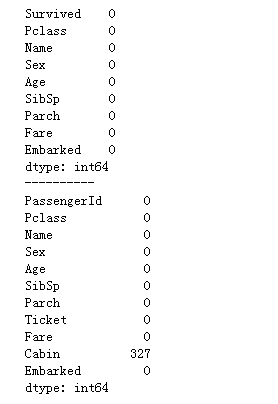
for dataset in data_cleaner:    
    #complete missing age with median
    dataset['Age'].fillna(dataset['Age'].median(), inplace = True)

    #complete embarked with mode
    dataset['Embarked'].fillna(dataset['Embarked'].mode()[0], inplace = True)

    #complete missing fare with median
    dataset['Fare'].fillna(dataset['Fare'].median(), inplace = True)
    
#delete the cabin feature/column and others previously stated to exclude in train dataset
drop_column = ['PassengerId','Cabin', 'Ticket']
data1.drop(drop_column, axis=1, inplace = True)

print(data1.isnull().sum())
print("-"*10)
print(data_val.isnull().sum())

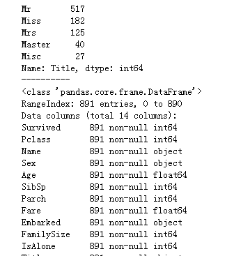
for dataset in data_cleaner:    
    #Discrete variables
    dataset['FamilySize'] = dataset ['SibSp'] + dataset['Parch'] + 1

    dataset['IsAlone'] = 1 #initialize to yes/1 is alone
    dataset['IsAlone'].loc[dataset['FamilySize'] > 1] = 0 # now update to no/0 if family size is greater than 1

    #quick and dirty code split title from name: http://www.pythonforbeginners.com/dictionary/python-split
    dataset['Title'] = dataset['Name'].str.split(", ", expand=True)[1].str.split(".", expand=True)[0]


    #Continuous variable bins; qcut vs cut: https://stackoverflow.com/questions/30211923/what-is-the-difference-between-pandas-qcut-and-pandas-cut
    #Fare Bins/Buckets using qcut or frequency bins: https://pandas.pydata.org/pandas-docs/stable/generated/pandas.qcut.html
    dataset['FareBin'] = pd.qcut(dataset['Fare'], 4)

    #Age Bins/Buckets using cut or value bins: https://pandas.pydata.org/pandas-docs/stable/generated/pandas.cut.html
    dataset['AgeBin'] = pd.cut(dataset['Age'].astype(int), 5)


    
#cleanup rare title names
#print(data1['Title'].value_counts())
stat_min = 10 #while small is arbitrary, we'll use the common minimum in statistics: http://nicholasjjackson.com/2012/03/08/sample-size-is-10-a-magic-number/
title_names = (data1['Title'].value_counts() < stat_min) #this will create a true false series with title name as index

#apply and lambda functions are quick and dirty code to find and replace with fewer lines of code: https://community.modeanalytics.com/python/tutorial/pandas-groupby-and-python-lambda-functions/
data1['Title'] = data1['Title'].apply(lambda x: 'Misc' if title_names.loc[x] == True else x)
print(data1['Title'].value_counts())
print("-"*10)


#preview data again
data1.info()
data_val.info()
data1.sample(10)

5.3 转换格式
我们将分类数据转换为虚拟变量以进行数学分析。 有多种方法可以对分类变量进行编码; 我们将使用sklearn和pandas函数。

在此步骤中，我们还将为数据建模定义x（独立/特征/解释/预测器/等）和y（依赖/目标/结果/响应/等）变量。

开发者文档:

• Categorical Encoding
• Sklearn LabelEncoder
• Sklearn OneHotEncoder
• Pandas Categorical dtype
• pandas.get_dummies

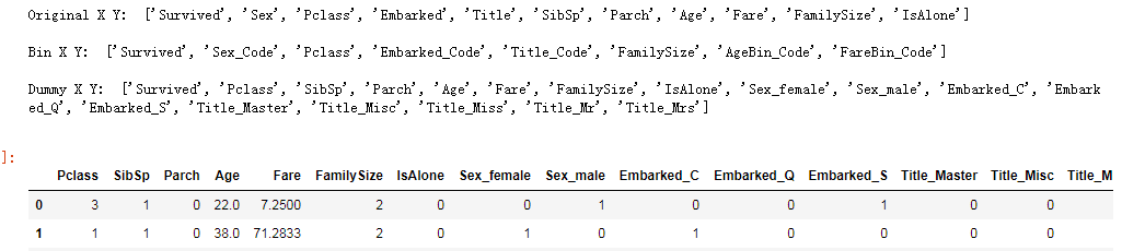
label = LabelEncoder()
for dataset in data_cleaner:    
    dataset['Sex_Code'] = label.fit_transform(dataset['Sex'])
    dataset['Embarked_Code'] = label.fit_transform(dataset['Embarked'])
    dataset['Title_Code'] = label.fit_transform(dataset['Title'])
    dataset['AgeBin_Code'] = label.fit_transform(dataset['AgeBin'])
    dataset['FareBin_Code'] = label.fit_transform(dataset['FareBin'])


#define y variable aka target/outcome
Target = ['Survived']

#define x variables for original features aka feature selection
data1_x = ['Sex','Pclass', 'Embarked', 'Title','SibSp', 'Parch', 'Age', 'Fare', 'FamilySize', 'IsAlone'] #pretty name/values for charts
data1_x_calc = ['Sex_Code','Pclass', 'Embarked_Code', 'Title_Code','SibSp', 'Parch', 'Age', 'Fare'] #coded for algorithm calculation
data1_xy =  Target + data1_x
print('Original X Y: ', data1_xy, '\n')


#define x variables for original w/bin features to remove continuous variables
data1_x_bin = ['Sex_Code','Pclass', 'Embarked_Code', 'Title_Code', 'FamilySize', 'AgeBin_Code', 'FareBin_Code']
data1_xy_bin = Target + data1_x_bin
print('Bin X Y: ', data1_xy_bin, '\n')


#define x and y variables for dummy features original
data1_dummy = pd.get_dummies(data1[data1_x])
data1_x_dummy = data1_dummy.columns.tolist()
data1_xy_dummy = Target + data1_x_dummy
print('Dummy X Y: ', data1_xy_dummy, '\n')



data1_dummy.head()

5.4 再次检查清理数据
现在我们已经清理了我们的数据，让我们做再次检查！

print('Train columns with null values: \n', data1.isnull().sum())
print("-"*10)
print (data1.info())
print("-"*10)

print('Test/Validation columns with null values: \n', data_val.isnull().sum())
print("-"*10)
print (data_val.info())
print("-"*10)

data_raw.describe(include = 'all')

 

 

5.5 拆分训练和测试数据
　　如前所述，提供测试的文件实际上是竞赛提交的验证数据。 因此，我们将使用sklearn函数将训练数据分成两个数据集; 75/25分裂。 这很重要，所以我们不会过度拟合（overfitting）我们的模型。 意思是，该算法对于给定子集是如此特定，它不能从同一数据集中准确地推广另一个子集。 重要的是我们的算法没有看到我们将用于测试的子集，因此它不会通过记忆答案来“欺骗”。 我们将使用sklearn的train_test_split函数。 在后面的部分中，我们还将使用sklearn的交叉验证函数(cross validation functions,)，将我们的数据集拆分为训练和测试数据建模比较。

#split train and test data with function defaults
#random_state -> seed or control random number generator: https://www.quora.com/What-is-seed-in-random-number-generation
train1_x, test1_x, train1_y, test1_y = model_selection.train_test_split(data1[data1_x_calc], data1[Target], random_state = 0)
train1_x_bin, test1_x_bin, train1_y_bin, test1_y_bin = model_selection.train_test_split(data1[data1_x_bin], data1[Target] , random_state = 0)
train1_x_dummy, test1_x_dummy, train1_y_dummy, test1_y_dummy = model_selection.train_test_split(data1_dummy[data1_x_dummy], data1[Target], random_state = 0)


print("Data1 Shape: {}".format(data1.shape))
print("Train1 Shape: {}".format(train1_x.shape))
print("Test1 Shape: {}".format(test1_x.shape))

train1_x_bin.head()

 

六、步骤4：进行探索性分析

　　现在我们的数据已经清理完毕，我们将使用描述性统计和图形化统计数据来探索我们的数据。 在这个阶段，你会发现自己对特征进行分类并确定它们与目标变量和彼此之间的相关性。

#Discrete Variable Correlation by Survival using
#group by aka pivot table: https://pandas.pydata.org/pandas-docs/stable/generated/pandas.DataFrame.groupby.html
for x in data1_x:
    if data1[x].dtype != 'float64' :
        print('Survival Correlation by:', x)
        print(data1[[x, Target[0]]].groupby(x, as_index=False).mean())
        print('-'*10, '\n')
        

#using crosstabs: https://pandas.pydata.org/pandas-docs/stable/generated/pandas.crosstab.html
print(pd.crosstab(data1['Title'],data1[Target[0]]))

 

#IMPORTANT: Intentionally plotted different ways for learning purposes only. 

#optional plotting w/pandas: https://pandas.pydata.org/pandas-docs/stable/visualization.html

#we will use matplotlib.pyplot: https://matplotlib.org/api/pyplot_api.html

#to organize our graphics will use figure: https://matplotlib.org/api/_as_gen/matplotlib.pyplot.figure.html#matplotlib.pyplot.figure
#subplot: https://matplotlib.org/api/_as_gen/matplotlib.pyplot.subplot.html#matplotlib.pyplot.subplot
#and subplotS: https://matplotlib.org/api/_as_gen/matplotlib.pyplot.subplots.html?highlight=matplotlib%20pyplot%20subplots#matplotlib.pyplot.subplots

#graph distribution of quantitative data
plt.figure(figsize=[16,12])

plt.subplot(231)
plt.boxplot(x=data1['Fare'], showmeans = True, meanline = True)
plt.title('Fare Boxplot')
plt.ylabel('Fare ($)')

plt.subplot(232)
plt.boxplot(data1['Age'], showmeans = True, meanline = True)
plt.title('Age Boxplot')
plt.ylabel('Age (Years)')

plt.subplot(233)
plt.boxplot(data1['FamilySize'], showmeans = True, meanline = True)
plt.title('Family Size Boxplot')
plt.ylabel('Family Size (#)')

plt.subplot(234)
plt.hist(x = [data1[data1['Survived']==1]['Fare'], data1[data1['Survived']==0]['Fare']], 
         stacked=True, color = ['g','r'],label = ['Survived','Dead'])
plt.title('Fare Histogram by Survival')
plt.xlabel('Fare ($)')
plt.ylabel('# of Passengers')
plt.legend()

plt.subplot(235)
plt.hist(x = [data1[data1['Survived']==1]['Age'], data1[data1['Survived']==0]['Age']], 
         stacked=True, color = ['g','r'],label = ['Survived','Dead'])
plt.title('Age Histogram by Survival')
plt.xlabel('Age (Years)')
plt.ylabel('# of Passengers')
plt.legend()

plt.subplot(236)
plt.hist(x = [data1[data1['Survived']==1]['FamilySize'], data1[data1['Survived']==0]['FamilySize']], 
         stacked=True, color = ['g','r'],label = ['Survived','Dead'])
plt.title('Family Size Histogram by Survival')
plt.xlabel('Family Size (#)')
plt.ylabel('# of Passengers')
plt.legend()

#we will use seaborn graphics for multi-variable comparison: https://seaborn.pydata.org/api.html

#graph individual features by survival
fig, saxis = plt.subplots(2, 3,figsize=(16,12))

sns.barplot(x = 'Embarked', y = 'Survived', data=data1, ax = saxis[0,0])
sns.barplot(x = 'Pclass', y = 'Survived', order=[1,2,3], data=data1, ax = saxis[0,1])
sns.barplot(x = 'IsAlone', y = 'Survived', order=[1,0], data=data1, ax = saxis[0,2])

sns.pointplot(x = 'FareBin', y = 'Survived',  data=data1, ax = saxis[1,0])
sns.pointplot(x = 'AgeBin', y = 'Survived',  data=data1, ax = saxis[1,1])
sns.pointplot(x = 'FamilySize', y = 'Survived', data=data1, ax = saxis[1,2])

 

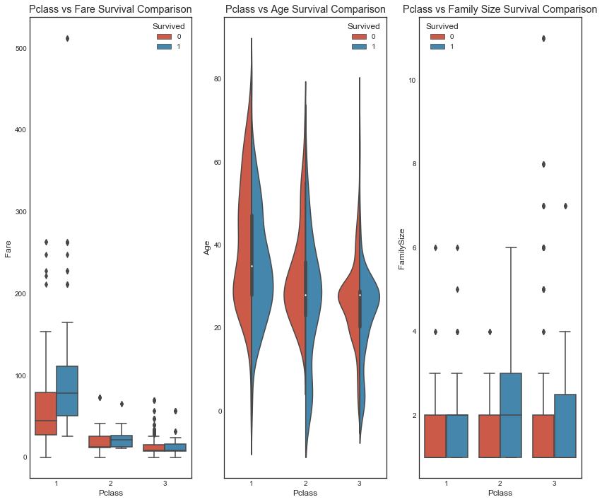
#graph distribution of qualitative data: Pclass
#we know class mattered in survival, now let's compare class and a 2nd feature
fig, (axis1,axis2,axis3) = plt.subplots(1,3,figsize=(14,12))

sns.boxplot(x = 'Pclass', y = 'Fare', hue = 'Survived', data = data1, ax = axis1)
axis1.set_title('Pclass vs Fare Survival Comparison')

sns.violinplot(x = 'Pclass', y = 'Age', hue = 'Survived', data = data1, split = True, ax = axis2)
axis2.set_title('Pclass vs Age Survival Comparison')

sns.boxplot(x = 'Pclass', y ='FamilySize', hue = 'Survived', data = data1, ax = axis3)
axis3.set_title('Pclass vs Family Size Survival Comparison')

 

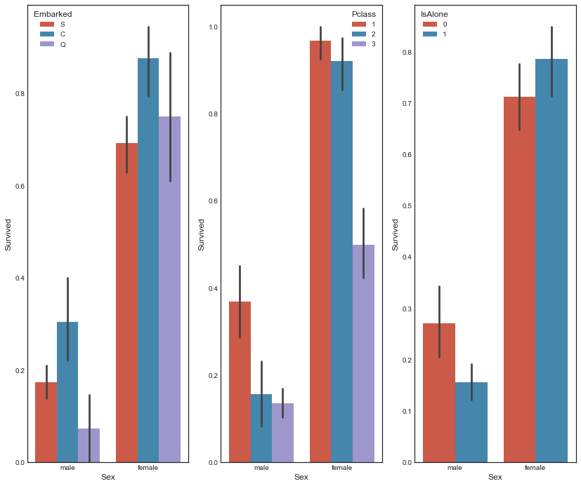
#graph distribution of qualitative data: Sex
#we know sex mattered in survival, now let's compare sex and a 2nd feature
fig, qaxis = plt.subplots(1,3,figsize=(14,12))

sns.barplot(x = 'Sex', y = 'Survived', hue = 'Embarked', data=data1, ax = qaxis[0])
axis1.set_title('Sex vs Embarked Survival Comparison')

sns.barplot(x = 'Sex', y = 'Survived', hue = 'Pclass', data=data1, ax  = qaxis[1])
axis1.set_title('Sex vs Pclass Survival Comparison')

sns.barplot(x = 'Sex', y = 'Survived', hue = 'IsAlone', data=data1, ax  = qaxis[2])
axis1.set_title('Sex vs IsAlone Survival Comparison')

#more side-by-side comparisons
fig, (maxis1, maxis2) = plt.subplots(1, 2,figsize=(14,12))

#how does family size factor with sex & survival compare
sns.pointplot(x="FamilySize", y="Survived", hue="Sex", data=data1,
              palette={"male": "blue", "female": "pink"},
              markers=["*", "o"], linestyles=["-", "--"], ax = maxis1)

#how does class factor with sex & survival compare
sns.pointplot(x="Pclass", y="Survived", hue="Sex", data=data1,
              palette={"male": "blue", "female": "pink"},
              markers=["*", "o"], linestyles=["-", "--"], ax = maxis2)

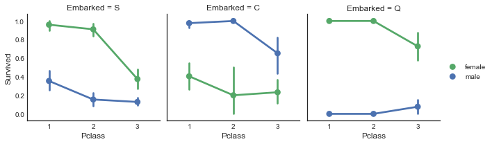
#how does embark port factor with class, sex, and survival compare
#facetgrid: https://seaborn.pydata.org/generated/seaborn.FacetGrid.html
e = sns.FacetGrid(data1, col = 'Embarked')
e.map(sns.pointplot, 'Pclass', 'Survived', 'Sex', ci=95.0, palette = 'deep')
e.add_legend()

#how does embark port factor with class, sex, and survival compare
#facetgrid: https://seaborn.pydata.org/generated/seaborn.FacetGrid.html

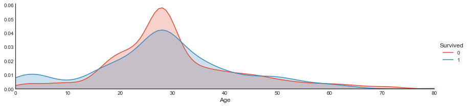
a = sns.FacetGrid( data1, hue = 'Survived', aspect=4 )
a.map(sns.kdeplot, 'Age', shade= True )
a.set(xlim=(0 , data1['Age'].max()))
a.add_legend()

#histogram comparison of sex, class, and age by survival

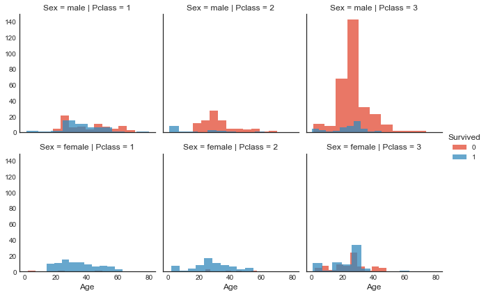
h = sns.FacetGrid(data1, row = 'Sex', col = 'Pclass', hue = 'Survived')
h.map(plt.hist, 'Age', alpha = .75)
h.add_legend()

#pair plots of entire dataset
pp = sns.pairplot(data1, hue = 'Survived', palette = 'deep', size=1.2, diag_kind = 'kde', diag_kws=dict(shade=True), plot_kws=dict(s=10) )
pp.set(xticklabels=[])

 

 

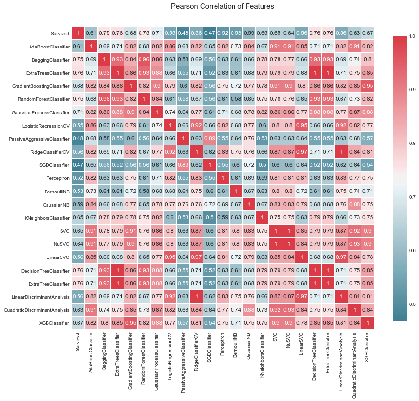
#correlation heatmap of dataset
def correlation_heatmap(df):
    _ , ax = plt.subplots(figsize =(14, 12))
    colormap = sns.diverging_palette(220, 10, as_cmap = True)
    
    _ = sns.heatmap(
        df.corr(), 
        cmap = colormap,
        square=True, 
        cbar_kws={'shrink':.9 }, 
        ax=ax,
        annot=True, 
        linewidths=0.1,vmax=1.0, linecolor='white',
        annot_kws={'fontsize':12 }
    )
    
    plt.title('Pearson Correlation of Features', y=1.05, size=15)

correlation_heatmap(data1)

 

 

七、步骤5：模型数据

　　数据科学是数学、统计学、计算机科学、和商业管理之间的多学科领域。大多数数据科学家来自三个领域之一，因此他们倾向于该学科。然而，数据科学就像一个三脚凳，没有一条腿比另一条腿更重要。因此，这一步将需要先进的数学知识。但不要担心，我们只需要一个高级概述，我们将在文章中介绍。此外，由于计算机科学的发展，很多繁重的工作都用计算机完成。因此，曾经需要数学或统计学研究生学位的问题，现在只需要几行代码。最后，我们需要一些商业头脑来思考问题。毕竟，就像训练宠物一样，它是向我们学习，需要我们一点一点引导。

　　机器学习（ML），顾名思义，就是教机器如何思考而不是思考什么。虽然这个话题和大数据已经存在了几十年，但它正变得比以往任何时候都更受欢迎，因为对于企业和专业人士而言，进入门槛较低。这既好又坏。这很好，因为这些算法现在可供更多人使用，可以解决现实世界中的更多问题。这很糟糕，因为进入门槛较低意味着，更多的人不会知道他们使用的工具，并且会得出错误的结论。以前，我曾经比喻过要求别人给你一把螺丝刀，他们会给你一把平头螺丝刀或最差的锤子。充其量，它表明完全缺乏理解。在最坏的情况下，它使项目变得很差;甚至最糟糕的是，得出错误的结论。所以，现在，我会告诉你该怎么做，最重要的是，为什么你这样做。

　　首先，你必须明白，机器学习的目的是解决人类的问题。机器学习可分为：监督学习，无监督学习和强化学习。监督学习是指通过向训练数据集提供包含正确答案的训练模型来训练模型的地方。无监督学习是使用不包含正确答案的训练数据集训练模型的地方。强化学习是前两者的混合体，其中模型没有立即给出正确的答案，但是在一系列事件之后加强学习。我们正在进行有监督的机器学习，因为我们通过提供一组特征及其相应的目标来训练我们的算法。然后，我们希望从同一数据集中为它提供一个新的子集，并且在预测精度方面具有相似的结果。

　　有许多机器学习算法，但它们可以简化为四类：分类，回归，聚类或降维，具体取决于您的目标变量和数据建模目标。本文中专注于分类和回归。我们可以概括出连续目标变量需要回归算法而离散目标变量需要分类算法。一方面注意，逻辑回归虽然名称中有回归，但实际上是一种分类算法。由于我们的问题是预测乘客是否幸存或未幸存，因此这是一个离散的目标变量。我们将使用sklearn库中的分类算法开始我们的分析。我们将使用交叉验证和评分指标，在后面的章节中讨论，以排名和比较我们的算法的性能。

机器学习模型选择：

• Sklearn Estimator Overview
• Sklearn Estimator Detail
• Choosing Estimator Mind Map
• Choosing Estimator Cheat Sheet

机器学习常见的分类算法：

• Ensemble Methods
• Generalized Linear Models (GLM)
• Naive Bayes
• Nearest Neighbors
• Support Vector Machines (SVM)
• Decision Trees
• Discriminant Analysis

那么，如何选择机器学习算法（MLA）？
　　重要提示：在数据建模方面，初学者的问题始终是“什么是最好的机器学习算法？”对此，初学者必须学习机器学习的免费午餐定理（No Free Lunch Theorem (NFLT)）。简而言之，NFLT指出，对于所有数据集，没有超级算法在所有情况下都能发挥最佳作用。因此，最好的方法是尝试多个工作量，调整它们，并根据您的具体情况进行比较。话虽如此，已经进行了一些很好的研究来比较算法，例如 Caruana & Niculescu-Mizil 2006， Ogutu et al. 2011NIH完成基因组选择， Fernandez-Delgado et al. 2014比较了来自17个家庭的179个分类器，并且还有一种思想流派认为，Thoma 2016 sklearn comparison, 更多的数据打败了更好的算法。

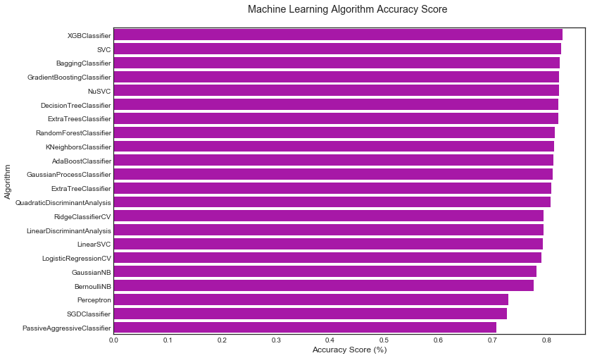
　　所有这些信息，初学者在哪里开始？我建议从树木，套袋，随机森林和提升（Trees, Bagging, Random Forests, and Boosting）开始。它们基本上是决策树的不同实现，这是最容易学习和理解的概念。与SVC相比，它们在下一节中也更容易调整。下面，我将概述如何运行和比较几个MLA，但这个内核的其余部分将侧重于通过决策树及其衍生物学习数据建模。

#Machine Learning Algorithm (MLA) Selection and Initialization
MLA = [
    #Ensemble Methods
    ensemble.AdaBoostClassifier(),
    ensemble.BaggingClassifier(),
    ensemble.ExtraTreesClassifier(),
    ensemble.GradientBoostingClassifier(),
    ensemble.RandomForestClassifier(),

    #Gaussian Processes
    gaussian_process.GaussianProcessClassifier(),
    
    #GLM
    linear_model.LogisticRegressionCV(),
    linear_model.PassiveAggressiveClassifier(),
    linear_model.RidgeClassifierCV(),
    linear_model.SGDClassifier(),
    linear_model.Perceptron(),
    
    #Navies Bayes
    naive_bayes.BernoulliNB(),
    naive_bayes.GaussianNB(),
    
    #Nearest Neighbor
    neighbors.KNeighborsClassifier(),
    
    #SVM
    svm.SVC(probability=True),
    svm.NuSVC(probability=True),
    svm.LinearSVC(),
    
    #Trees    
    tree.DecisionTreeClassifier(),
    tree.ExtraTreeClassifier(),
    
    #Discriminant Analysis
    discriminant_analysis.LinearDiscriminantAnalysis(),
    discriminant_analysis.QuadraticDiscriminantAnalysis(),

    
    #xgboost: http://xgboost.readthedocs.io/en/latest/model.html
    XGBClassifier()    
    ]



#split dataset in cross-validation with this splitter class: http://scikit-learn.org/stable/modules/generated/sklearn.model_selection.ShuffleSplit.html#sklearn.model_selection.ShuffleSplit
#note: this is an alternative to train_test_split
cv_split = model_selection.ShuffleSplit(n_splits = 10, test_size = .3, train_size = .6, random_state = 0 ) # run model 10x with 60/30 split intentionally leaving out 10%

#create table to compare MLA metrics
MLA_columns = ['MLA Name', 'MLA Parameters','MLA Train Accuracy Mean', 'MLA Test Accuracy Mean', 'MLA Test Accuracy 3*STD' ,'MLA Time']
MLA_compare = pd.DataFrame(columns = MLA_columns)

#create table to compare MLA predictions
MLA_predict = data1[Target]

#index through MLA and save performance to table
row_index = 0
for alg in MLA:

    #set name and parameters
    MLA_name = alg.__class__.__name__
    MLA_compare.loc[row_index, 'MLA Name'] = MLA_name
    MLA_compare.loc[row_index, 'MLA Parameters'] = str(alg.get_params())
    
    #score model with cross validation: http://scikit-learn.org/stable/modules/generated/sklearn.model_selection.cross_validate.html#sklearn.model_selection.cross_validate
    cv_results = model_selection.cross_validate(alg, data1[data1_x_bin], data1[Target], cv  = cv_split)

    MLA_compare.loc[row_index, 'MLA Time'] = cv_results['fit_time'].mean()
    MLA_compare.loc[row_index, 'MLA Train Accuracy Mean'] = cv_results['train_score'].mean()
    MLA_compare.loc[row_index, 'MLA Test Accuracy Mean'] = cv_results['test_score'].mean()   
    #if this is a non-bias random sample, then +/-3 standard deviations (std) from the mean, should statistically capture 99.7% of the subsets
    MLA_compare.loc[row_index, 'MLA Test Accuracy 3*STD'] = cv_results['test_score'].std()*3   #let's know the worst that can happen!
    

    #save MLA predictions - see section 6 for usage
    alg.fit(data1[data1_x_bin], data1[Target])
    MLA_predict[MLA_name] = alg.predict(data1[data1_x_bin])
    
    row_index+=1

    
#print and sort table: https://pandas.pydata.org/pandas-docs/stable/generated/pandas.DataFrame.sort_values.html
MLA_compare.sort_values(by = ['MLA Test Accuracy Mean'], ascending = False, inplace = True)
MLA_compare
#MLA_predict

#barplot using https://seaborn.pydata.org/generated/seaborn.barplot.html
sns.barplot(x='MLA Test Accuracy Mean', y = 'MLA Name', data = MLA_compare, color = 'm')

#prettify using pyplot: https://matplotlib.org/api/pyplot_api.html
plt.title('Machine Learning Algorithm Accuracy Score \n')
plt.xlabel('Accuracy Score (%)')
plt.ylabel('Algorithm')

 

八、评估模型性能

　　让我们回顾一下，通过一些基本的数据清理，分析和机器学习算法（MLA），我们能够以大约82％的准确度预测乘客的生存。 几行代码也不错。 但我们一直在问的问题是，我们能投入更多时间，更重要的是获得更多的投资回报率吗？ 例如，如果我们只是将准确度提高0.1，那么开发真的值3个月。 如果你在研究中工作，答案是肯定的，但如果你在商业中工作，答案肯定是否定的。 因此，在改进模型时请记住这一点。

NOTE：确定基线准确度
　　在我们决定如何使我们的模型更好之前，让我们确定我们的模型是否值得保留。要做到这一点，我们必须回到数据科学的基础.我们知道这是一个二元问题，因为只有两种可能的结果;乘客幸存或死亡。所以，把它想象成硬币翻转问题。如果你有一个公平的硬币并且猜到了头或尾，那么你有50％的机会猜测正确。所以，让我们将50％设为最差的模特表现;因为低于那个，那么为什么我只需要翻硬币就需要你？

　　所以，没有关于数据集的信息，我们总是可以得到50％的二进制问题。但是我们有关于数据集的信息，所以我们应该能够做得更好。我们知道1,502 / 2,224或67.5％的人死亡。因此，如果我们只是预测最常见的事件，那100％的人死亡，那么我们使用67.5％的概率。所以，让我们将68％设置为糟糕的模型性能，因为再次，低于此值，那么为什么我需要你，当我可以预测使用最频繁的事件。

NOTE：如何创建自己的模型
　　我们的准确性正在提高，但我们可以做得更好吗？我们的数据中是否有任何信号？为了说明这一点，我们将构建自己的决策树模型，因为它最容易构思并需要简单的加法和乘法计算。创建决策树时，您需要提出分段目标响应的问题，将幸存的1和死亡0放入同类子组中。这是科学和艺术的一部分，所以让我们玩21个问题的游戏，告诉你它是如何工作的。如果您想自己动手，请下载火车数据集并导入Excel。创建一个数据透视表，其中包含列中的生存，值的行数和计数，以及行中下面描述的功能。

　　请记住，游戏的名称是使用决策树模型创建子组，以便在一个存储桶中存活1，在另一个存储桶中存在死0。我们的经验法则是多数规则。意思是，如果大部分或50％或更多存活，那么我们亚组中的每个人都存活 1，但如果50％或更少存活，那么如果我们子组中的每个人都死亡/0。此外，如果子组小于10或我们的模型精度平稳或降低，我们将停止。

问题1：你是泰坦尼克号吗？如果是，则大部分（62％）死亡。请注意，我们的样本存活率与我们68％的人口不同。尽管如此，如果我们假设每个人都死了，我们的样本准确率为62％。

问题2：你是男性还是女性？男性，大多数（81％）死亡。女性，大多数（74％）幸免于难。给我们79％的准确率。

问题3A（沿着女性分支进行计数= 314）：您是第1,2或3级？ 1级，大多数（97％）存活，2级，大部分（92％）存活。由于死子组小于10，我们将停止进入该分支。 3级，甚至是50-50分。没有获得改进我们模型的新信息。

问题4A（沿着女性3级分支，计数= 144）：您是从C，Q还是S出发？我们获得了一些信息。 C和Q，大部分仍然存活，所以没有变化。此外，死子组小于10，所以我们将停止。 S，大多数人（63％）死亡。所以，我们将改变女性，第3类，让S从假设幸存下来，假设他们死了。我们的模型精度提高到81％。

问题5A（从女性班级3开始走向S分支，计数= 88）：到目前为止，看起来我们做出了很好的决定。添加另一个级别似乎没有获得更多信息。该小组55死亡，33人幸存，因为多数人死亡，我们需要找到一个信号来识别33或一个小组，将他们从死亡变为幸存，并提高我们的模型准确性。我们可以玩我们的功能。我找到的一个是0-8的票价，大多数幸存下来。这是一个11-9的小样本，但经常用于统计。我们略微提高了准确度，但没有太多让我们超过82％。所以，我们会在这里停下来。

问题3B（沿着男性分支进行计数= 577）：回到问题2，我们知道大多数男性死亡。因此，我们正在寻找一种能够识别大多数幸存下来的子群的功能。令人惊讶的是，上课或甚至开始并没有像女性那样重要，但是头衔确实让我们达到了82％。猜测并检查其他功能，似乎没有一个让我们超过82％。所以，我们暂时停在这里。

你做到了，信息很少，我们的准确率达到了82％。在最糟糕的，坏的，好的，更好的和最好的规模上，我们将82％设置为好，因为它是一个简单的模型，可以产生不错的结果。但问题仍然存在，我们能比手工制作的模型更好吗？

在我们开始之前，让我们编写上面刚写的内容。请注意，这是由“手”创建的手动过程。您不必这样做，但在开始使用MLA之前了解它非常重要。在微积分考试中将MLA想象成TI-89计算器。它非常强大，可以帮助您完成大量繁重的工作。但如果你不知道你在考试中做了什么，计算器，甚至是TI-89，都不会帮助你通过。所以，明智地研究下一节。

参考：: Cross-Validation and Decision Tree Tutorial

#le/generated/pandas.DataFrame.iterrows.html
for index, row in data1.iterrows(): 
    #random number generator: https://docs.python.org/2/library/random.html
    if random.random() > .5:     # Random float x, 0.0 <= x < 1.0    
        data1.set_value(index, 'Random_Predict', 1) #predict survived/1
    else: 
        data1.set_value(index, 'Random_Predict', 0) #predict died/0
    

#score random guess of survival. Use shortcut 1 = Right Guess and 0 = Wrong Guess
#the mean of the column will then equal the accuracy
data1['Random_Score'] = 0 #assume prediction wrong
data1.loc[(data1['Survived'] == data1['Random_Predict']), 'Random_Score'] = 1 #set to 1 for correct prediction
print('Coin Flip Model Accuracy: {:.2f}%'.format(data1['Random_Score'].mean()*100))

#we can also use scikit's accuracy_score function to save us a few lines of code
#http://scikit-learn.org/stable/modules/generated/sklearn.metrics.accuracy_score.html#sklearn.metrics.accuracy_score
print('Coin Flip Model Accuracy w/SciKit: {:.2f}%'.format(metrics.accuracy_score(data1['Survived'], data1['Random_Predict'])*100))

 

#e.groupby.html
pivot_female = data1[data1.Sex=='female'].groupby(['Sex','Pclass', 'Embarked','FareBin'])['Survived'].mean()
print('Survival Decision Tree w/Female Node: \n',pivot_female)

pivot_male = data1[data1.Sex=='male'].groupby(['Sex','Title'])['Survived'].mean()
print('\n\nSurvival Decision Tree w/Male Node: \n',pivot_male)

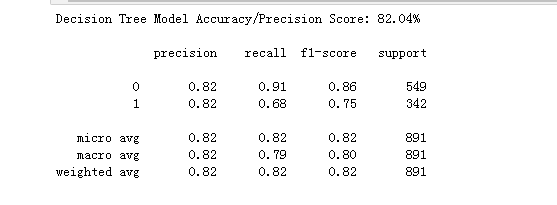
def mytree(df):
    
    #initialize table to store predictions
    Model = pd.DataFrame(data = {'Predict':[]})
    male_title = ['Master'] #survived titles

    for index, row in df.iterrows():

        #Question 1: Were you on the Titanic; majority died
        Model.loc[index, 'Predict'] = 0

        #Question 2: Are you female; majority survived
        if (df.loc[index, 'Sex'] == 'female'):
                  Model.loc[index, 'Predict'] = 1

        #Question 3A Female - Class and Question 4 Embarked gain minimum information

        #Question 5B Female - FareBin; set anything less than .5 in female node decision tree back to 0       
        if ((df.loc[index, 'Sex'] == 'female') & 
            (df.loc[index, 'Pclass'] == 3) & 
            (df.loc[index, 'Embarked'] == 'S')  &
            (df.loc[index, 'Fare'] > 8)

           ):
                  Model.loc[index, 'Predict'] = 0

        #Question 3B Male: Title; set anything greater than .5 to 1 for majority survived
        if ((df.loc[index, 'Sex'] == 'male') &
            (df.loc[index, 'Title'] in male_title)
            ):
            Model.loc[index, 'Predict'] = 1
        
        
    return Model


#model data
Tree_Predict = mytree(data1)
print('Decision Tree Model Accuracy/Precision Score: {:.2f}%\n'.format(metrics.accuracy_score(data1['Survived'], Tree_Predict)*100))

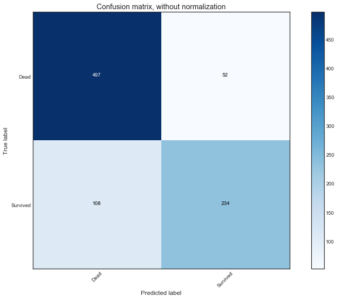
#model data
Tree_Predict = mytree(data1)
print('Decision Tree Model Accuracy/Precision Score: {:.2f}%\n'.format(metrics.accuracy_score(data1['Survived'], Tree_Predict)*100))

#assification_report.html#sklearn.metrics.classification_report
#Where recall score = (true positives)/(true positive + false negative) w/1 being best:http://scikit-learn.org/stable/modules/generated/sklearn.metrics.recall_score.html#sklearn.metrics.recall_score
#And F1 score = weighted average of precision and recall w/1 being best: http://scikit-learn.org/stable/modules/generated/sklearn.metrics.f1_score.html#sklearn.metrics.f1_score
print(metrics.classification_report(data1['Survived'], Tree_Predict))

import itertools
def plot_confusion_matrix(cm, classes,
                          normalize=False,
                          title='Confusion matrix',
                          cmap=plt.cm.Blues):
    """
    This function prints and plots the confusion matrix.
    Normalization can be applied by setting `normalize=True`.
    """
    if normalize:
        cm = cm.astype('float') / cm.sum(axis=1)[:, np.newaxis]
        print("Normalized confusion matrix")
    else:
        print('Confusion matrix, without normalization')

    print(cm)

    plt.imshow(cm, interpolation='nearest', cmap=cmap)
    plt.title(title)
    plt.colorbar()
    tick_marks = np.arange(len(classes))
    plt.xticks(tick_marks, classes, rotation=45)
    plt.yticks(tick_marks, classes)

    fmt = '.2f' if normalize else 'd'
    thresh = cm.max() / 2.
    for i, j in itertools.product(range(cm.shape[0]), range(cm.shape[1])):
        plt.text(j, i, format(cm[i, j], fmt),
                 horizontalalignment="center",
                 color="white" if cm[i, j] > thresh else "black")

    plt.tight_layout()
    plt.ylabel('True label')
    plt.xlabel('Predicted label')

# Compute confusion matrix
cnf_matrix = metrics.confusion_matrix(data1['Survived'], Tree_Predict)
np.set_printoptions(precision=2)

class_names = ['Dead', 'Survived']
# Plot non-normalized confusion matrix
plt.figure()
plot_confusion_matrix(cnf_matrix, classes=class_names,
                      title='Confusion matrix, without normalization')

# Plot normalized confusion matrix
plt.figure()
plot_confusion_matrix(cnf_matrix, classes=class_names, normalize=True, 
                      title='Normalized confusion matrix')

8.1 交叉验证（CV）的模型性能
　　在步骤5.0中，我们使用sklearn cross_validate函数来训练，测试和评分我们的模型性能。

　　请记住，重要的是我们使用不同的火车数据子集来构建我们的模型和测试数据来评估我们的模型。否则，我们的模型将被过度装配。意思是它已经看到了“预测”数据的好处，但是在预测未见到的数据方面很糟糕;这根本不是预测。这就像在学校测验中作弊获得100％，但是当你参加考试时，你失败了，因为你从未真正学到任何东西。机器学习也是如此。

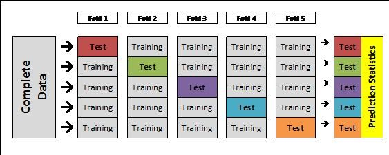
　　CV基本上是一种快捷方式，可以多次拆分和评分我们的模型，因此我们可以了解它对未见数据的执行情况。它在计算机处理方面要贵一些，但它很重要，所以我们不会获得虚假的信心。这在Kaggle比赛或任何需要避免一致性和意外的用例中很有用。

　　除了CV之外，我们还使用了定制的 sklearn train test splitter,，以便在我们的测试评分中获得更多随机性。下面是默认CV拆分的图像。

九、具有超参数的调整模型

　　当我们使用sklearn决策树（DT）分类器时(sklearn Decision Tree (DT) Classifier)，我们接受了所有函数默认值。 这样就有机会了解各种超参数设置如何改变模型的准确性。 （ (Click here to learn more about parameters vs hyper-parameters.)。）

　　但是，为了调整模型，我们需要真正理解它。 这就是为什么我花时间在前几节中向您展示预测是如何工作的。 现在让我们更多地了解我们的DT算法。

参考：sklearn

 关于决策树的优缺点，参见我写的关于决策树的文章。

　　以下是可用的超参数和定义：

class sklearn.tree.DecisionTreeClassifier（criterion ='gini'，splitter ='best'，max_depth = None，min_samples_split = 2，min_samples_leaf = 1，min_weight_fraction_leaf = 0.0，max_features = None，random_state = None，max_leaf_nodes = None，min_impurity_decrease = 0.0 ，min_impurity_split = None，class_weight = None，presort = False）

　　我们将使用ParameterGrid, GridSearchCV，和自定义的sklearn评分来调整我们的模型; 单击此处以了解有关ROC_AUC分数的更多信息（ sklearn scoring; click here to learn more about ROC_AUC scores）。 然后我们将使用graphviz.可视化我们的树。 单击此处以了解有关ROC_AUC分数的更多信息  （Click here to learn more about ROC_AUC scores.）。

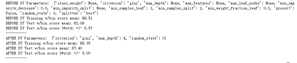
#base model
dtree = tree.DecisionTreeClassifier(random_state = 0)
base_results = model_selection.cross_validate(dtree, data1[data1_x_bin], data1[Target], cv  = cv_split)
dtree.fit(data1[data1_x_bin], data1[Target])

print('BEFORE DT Parameters: ', dtree.get_params())
print("BEFORE DT Training w/bin score mean: {:.2f}". format(base_results['train_score'].mean()*100)) 
print("BEFORE DT Test w/bin score mean: {:.2f}". format(base_results['test_score'].mean()*100))
print("BEFORE DT Test w/bin score 3*std: +/- {:.2f}". format(base_results['test_score'].std()*100*3))
#print("BEFORE DT Test w/bin set score min: {:.2f}". format(base_results['test_score'].min()*100))
print('-'*10)


#tune hyper-parameters: http://scikit-learn.org/stable/modules/generated/sklearn.tree.DecisionTreeClassifier.html#sklearn.tree.DecisionTreeClassifier
param_grid = {'criterion': ['gini', 'entropy'],  #scoring methodology; two supported formulas for calculating information gain - default is gini
              #'splitter': ['best', 'random'], #splitting methodology; two supported strategies - default is best
              'max_depth': [2,4,6,8,10,None], #max depth tree can grow; default is none
              #'min_samples_split': [2,5,10,.03,.05], #minimum subset size BEFORE new split (fraction is % of total); default is 2
              #'min_samples_leaf': [1,5,10,.03,.05], #minimum subset size AFTER new split split (fraction is % of total); default is 1
              #'max_features': [None, 'auto'], #max features to consider when performing split; default none or all
              'random_state': [0] #seed or control random number generator: https://www.quora.com/What-is-seed-in-random-number-generation
             }

#print(list(model_selection.ParameterGrid(param_grid)))

#choose best model with grid_search: #http://scikit-learn.org/stable/modules/grid_search.html#grid-search
#http://scikit-learn.org/stable/auto_examples/model_selection/plot_grid_search_digits.html
tune_model = model_selection.GridSearchCV(tree.DecisionTreeClassifier(), param_grid=param_grid, scoring = 'roc_auc', cv = cv_split)
tune_model.fit(data1[data1_x_bin], data1[Target])

#print(tune_model.cv_results_.keys())
#print(tune_model.cv_results_['params'])
print('AFTER DT Parameters: ', tune_model.best_params_)
#print(tune_model.cv_results_['mean_train_score'])
print("AFTER DT Training w/bin score mean: {:.2f}". format(tune_model.cv_results_['mean_train_score'][tune_model.best_index_]*100)) 
#print(tune_model.cv_results_['mean_test_score'])
print("AFTER DT Test w/bin score mean: {:.2f}". format(tune_model.cv_results_['mean_test_score'][tune_model.best_index_]*100))
print("AFTER DT Test w/bin score 3*std: +/- {:.2f}". format(tune_model.cv_results_['std_test_score'][tune_model.best_index_]*100*3))
print('-'*10)


#duplicates gridsearchcv
#tune_results = model_selection.cross_validate(tune_model, data1[data1_x_bin], data1[Target], cv  = cv_split)

#print('AFTER DT Parameters: ', tune_model.best_params_)
#print("AFTER DT Training w/bin set score mean: {:.2f}". format(tune_results['train_score'].mean()*100)) 
#print("AFTER DT Test w/bin set score mean: {:.2f}". format(tune_results['test_score'].mean()*100))
#print("AFTER DT Test w/bin set score min: {:.2f}". format(tune_results['test_score'].min()*100))
#print('-'*10)

十、具有特征选择的调整模型

　　如开头所述，变量越多，并不意味着模型越好，但正确的预测变量确实如此。 因此，数据建模的另一个步骤是特征选择。 Sklearn有几个选项，我们将使用带有交叉验证（CV）的递归特征消除（RFE）（ recursive feature elimination (RFE) with cross validation (CV).）。

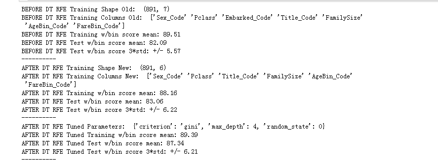
#base model
print('BEFORE DT RFE Training Shape Old: ', data1[data1_x_bin].shape) 
print('BEFORE DT RFE Training Columns Old: ', data1[data1_x_bin].columns.values)

print("BEFORE DT RFE Training w/bin score mean: {:.2f}". format(base_results['train_score'].mean()*100)) 
print("BEFORE DT RFE Test w/bin score mean: {:.2f}". format(base_results['test_score'].mean()*100))
print("BEFORE DT RFE Test w/bin score 3*std: +/- {:.2f}". format(base_results['test_score'].std()*100*3))
print('-'*10)



#feature selection
dtree_rfe = feature_selection.RFECV(dtree, step = 1, scoring = 'accuracy', cv = cv_split)
dtree_rfe.fit(data1[data1_x_bin], data1[Target])

#transform x&y to reduced features and fit new model
#alternative: can use pipeline to reduce fit and transform steps: http://scikit-learn.org/stable/modules/generated/sklearn.pipeline.Pipeline.html
X_rfe = data1[data1_x_bin].columns.values[dtree_rfe.get_support()]
rfe_results = model_selection.cross_validate(dtree, data1[X_rfe], data1[Target], cv  = cv_split)

#print(dtree_rfe.grid_scores_)
print('AFTER DT RFE Training Shape New: ', data1[X_rfe].shape) 
print('AFTER DT RFE Training Columns New: ', X_rfe)

print("AFTER DT RFE Training w/bin score mean: {:.2f}". format(rfe_results['train_score'].mean()*100)) 
print("AFTER DT RFE Test w/bin score mean: {:.2f}". format(rfe_results['test_score'].mean()*100))
print("AFTER DT RFE Test w/bin score 3*std: +/- {:.2f}". format(rfe_results['test_score'].std()*100*3))
print('-'*10)


#tune rfe model
rfe_tune_model = model_selection.GridSearchCV(tree.DecisionTreeClassifier(), param_grid=param_grid, scoring = 'roc_auc', cv = cv_split)
rfe_tune_model.fit(data1[X_rfe], data1[Target])

#print(rfe_tune_model.cv_results_.keys())
#print(rfe_tune_model.cv_results_['params'])
print('AFTER DT RFE Tuned Parameters: ', rfe_tune_model.best_params_)
#print(rfe_tune_model.cv_results_['mean_train_score'])
print("AFTER DT RFE Tuned Training w/bin score mean: {:.2f}". format(rfe_tune_model.cv_results_['mean_train_score'][tune_model.best_index_]*100)) 
#print(rfe_tune_model.cv_results_['mean_test_score'])
print("AFTER DT RFE Tuned Test w/bin score mean: {:.2f}". format(rfe_tune_model.cv_results_['mean_test_score'][tune_model.best_index_]*100))
print("AFTER DT RFE Tuned Test w/bin score 3*std: +/- {:.2f}". format(rfe_tune_model.cv_results_['std_test_score'][tune_model.best_index_]*100*3))
print('-'*10)

#Graph MLA version of Decision Tree: http://scikit-learn.org/stable/modules/generated/sklearn.tree.export_graphviz.html
import graphviz 
dot_data = tree.export_graphviz(dtree, out_file=None, 
                                feature_names = data1_x_bin, class_names = True,
                                filled = True, rounded = True)
graph = graphviz.Source(dot_data) 
graph

十一、步骤6：验证和实施

下一步是使用验证数据准备提交。

#compare algorithm predictions with each other, where 1 = exactly similar and 0 = exactly opposite
#there are some 1's, but enough blues and light reds to create a "super algorithm" by combining them
correlation_heatmap(MLA_predict)

 

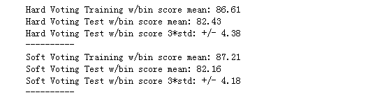
#why choose one model, when you can pick them all with voting classifier
#http://scikit-learn.org/stable/modules/generated/sklearn.ensemble.VotingClassifier.html
#removed models w/o attribute 'predict_proba' required for vote classifier and models with a 1.0 correlation to another model
vote_est = [
    #Ensemble Methods: http://scikit-learn.org/stable/modules/ensemble.html
    ('ada', ensemble.AdaBoostClassifier()),
    ('bc', ensemble.BaggingClassifier()),
    ('etc',ensemble.ExtraTreesClassifier()),
    ('gbc', ensemble.GradientBoostingClassifier()),
    ('rfc', ensemble.RandomForestClassifier()),

    #Gaussian Processes: http://scikit-learn.org/stable/modules/gaussian_process.html#gaussian-process-classification-gpc
    ('gpc', gaussian_process.GaussianProcessClassifier()),
    
    #GLM: http://scikit-learn.org/stable/modules/linear_model.html#logistic-regression
    ('lr', linear_model.LogisticRegressionCV()),
    
    #Navies Bayes: http://scikit-learn.org/stable/modules/naive_bayes.html
    ('bnb', naive_bayes.BernoulliNB()),
    ('gnb', naive_bayes.GaussianNB()),
    
    #Nearest Neighbor: http://scikit-learn.org/stable/modules/neighbors.html
    ('knn', neighbors.KNeighborsClassifier()),
    
    #SVM: http://scikit-learn.org/stable/modules/svm.html
    ('svc', svm.SVC(probability=True)),
    
    #xgboost: http://xgboost.readthedocs.io/en/latest/model.html
   ('xgb', XGBClassifier())

]


#Hard Vote or majority rules
vote_hard = ensemble.VotingClassifier(estimators = vote_est , voting = 'hard')
vote_hard_cv = model_selection.cross_validate(vote_hard, data1[data1_x_bin], data1[Target], cv  = cv_split)
vote_hard.fit(data1[data1_x_bin], data1[Target])

print("Hard Voting Training w/bin score mean: {:.2f}". format(vote_hard_cv['train_score'].mean()*100)) 
print("Hard Voting Test w/bin score mean: {:.2f}". format(vote_hard_cv['test_score'].mean()*100))
print("Hard Voting Test w/bin score 3*std: +/- {:.2f}". format(vote_hard_cv['test_score'].std()*100*3))
print('-'*10)


#Soft Vote or weighted probabilities
vote_soft = ensemble.VotingClassifier(estimators = vote_est , voting = 'soft')
vote_soft_cv = model_selection.cross_validate(vote_soft, data1[data1_x_bin], data1[Target], cv  = cv_split)
vote_soft.fit(data1[data1_x_bin], data1[Target])

print("Soft Voting Training w/bin score mean: {:.2f}". format(vote_soft_cv['train_score'].mean()*100)) 
print("Soft Voting Test w/bin score mean: {:.2f}". format(vote_soft_cv['test_score'].mean()*100))
print("Soft Voting Test w/bin score 3*std: +/- {:.2f}". format(vote_soft_cv['test_score'].std()*100*3))
print('-'*10)

 

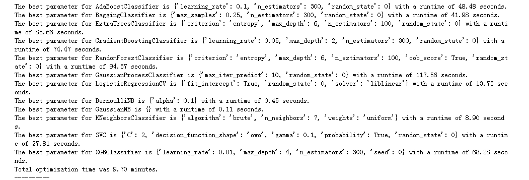
#WARNING: Running is very computational intensive and time expensive.
#Code is written for experimental/developmental purposes and not production ready!


#Hyperparameter Tune with GridSearchCV: http://scikit-learn.org/stable/modules/generated/sklearn.model_selection.GridSearchCV.html
grid_n_estimator = [10, 50, 100, 300]
grid_ratio = [.1, .25, .5, .75, 1.0]
grid_learn = [.01, .03, .05, .1, .25]
grid_max_depth = [2, 4, 6, 8, 10, None]
grid_min_samples = [5, 10, .03, .05, .10]
grid_criterion = ['gini', 'entropy']
grid_bool = [True, False]
grid_seed = [0]


grid_param = [
            [{
            #AdaBoostClassifier - http://scikit-learn.org/stable/modules/generated/sklearn.ensemble.AdaBoostClassifier.html
            'n_estimators': grid_n_estimator, #default=50
            'learning_rate': grid_learn, #default=1
            #'algorithm': ['SAMME', 'SAMME.R'], #default=’SAMME.R
            'random_state': grid_seed
            }],
       
    
            [{
            #BaggingClassifier - http://scikit-learn.org/stable/modules/generated/sklearn.ensemble.BaggingClassifier.html#sklearn.ensemble.BaggingClassifier
            'n_estimators': grid_n_estimator, #default=10
            'max_samples': grid_ratio, #default=1.0
            'random_state': grid_seed
             }],

    
            [{
            #ExtraTreesClassifier - http://scikit-learn.org/stable/modules/generated/sklearn.ensemble.ExtraTreesClassifier.html#sklearn.ensemble.ExtraTreesClassifier
            'n_estimators': grid_n_estimator, #default=10
            'criterion': grid_criterion, #default=”gini”
            'max_depth': grid_max_depth, #default=None
            'random_state': grid_seed
             }],


            [{
            #GradientBoostingClassifier - http://scikit-learn.org/stable/modules/generated/sklearn.ensemble.GradientBoostingClassifier.html#sklearn.ensemble.GradientBoostingClassifier
            #'loss': ['deviance', 'exponential'], #default=’deviance’
            'learning_rate': [.05], #default=0.1 -- 12/31/17 set to reduce runtime -- The best parameter for GradientBoostingClassifier is {'learning_rate': 0.05, 'max_depth': 2, 'n_estimators': 300, 'random_state': 0} with a runtime of 264.45 seconds.
            'n_estimators': [300], #default=100 -- 12/31/17 set to reduce runtime -- The best parameter for GradientBoostingClassifier is {'learning_rate': 0.05, 'max_depth': 2, 'n_estimators': 300, 'random_state': 0} with a runtime of 264.45 seconds.
            #'criterion': ['friedman_mse', 'mse', 'mae'], #default=”friedman_mse”
            'max_depth': grid_max_depth, #default=3   
            'random_state': grid_seed
             }],

    
            [{
            #RandomForestClassifier - http://scikit-learn.org/stable/modules/generated/sklearn.ensemble.RandomForestClassifier.html#sklearn.ensemble.RandomForestClassifier
            'n_estimators': grid_n_estimator, #default=10
            'criterion': grid_criterion, #default=”gini”
            'max_depth': grid_max_depth, #default=None
            'oob_score': [True], #default=False -- 12/31/17 set to reduce runtime -- The best parameter for RandomForestClassifier is {'criterion': 'entropy', 'max_depth': 6, 'n_estimators': 100, 'oob_score': True, 'random_state': 0} with a runtime of 146.35 seconds.
            'random_state': grid_seed
             }],
    
            [{    
            #GaussianProcessClassifier
            'max_iter_predict': grid_n_estimator, #default: 100
            'random_state': grid_seed
            }],
        
    
            [{
            #LogisticRegressionCV - http://scikit-learn.org/stable/modules/generated/sklearn.linear_model.LogisticRegressionCV.html#sklearn.linear_model.LogisticRegressionCV
            'fit_intercept': grid_bool, #default: True
            #'penalty': ['l1','l2'],
            'solver': ['newton-cg', 'lbfgs', 'liblinear', 'sag', 'saga'], #default: lbfgs
            'random_state': grid_seed
             }],
            
    
            [{
            #BernoulliNB - http://scikit-learn.org/stable/modules/generated/sklearn.naive_bayes.BernoulliNB.html#sklearn.naive_bayes.BernoulliNB
            'alpha': grid_ratio, #default: 1.0
             }],
    
    
            #GaussianNB - 
            [{}],
    
            [{
            #KNeighborsClassifier - http://scikit-learn.org/stable/modules/generated/sklearn.neighbors.KNeighborsClassifier.html#sklearn.neighbors.KNeighborsClassifier
            'n_neighbors': [1,2,3,4,5,6,7], #default: 5
            'weights': ['uniform', 'distance'], #default = ‘uniform’
            'algorithm': ['auto', 'ball_tree', 'kd_tree', 'brute']
            }],
            
    
            [{
            #SVC - http://scikit-learn.org/stable/modules/generated/sklearn.svm.SVC.html#sklearn.svm.SVC
            #http://blog.hackerearth.com/simple-tutorial-svm-parameter-tuning-python-r
            #'kernel': ['linear', 'poly', 'rbf', 'sigmoid'],
            'C': [1,2,3,4,5], #default=1.0
            'gamma': grid_ratio, #edfault: auto
            'decision_function_shape': ['ovo', 'ovr'], #default:ovr
            'probability': [True],
            'random_state': grid_seed
             }],

    
            [{
            #XGBClassifier - http://xgboost.readthedocs.io/en/latest/parameter.html
            'learning_rate': grid_learn, #default: .3
            'max_depth': [1,2,4,6,8,10], #default 2
            'n_estimators': grid_n_estimator, 
            'seed': grid_seed  
             }]   
        ]



start_total = time.perf_counter() #https://docs.python.org/3/library/time.html#time.perf_counter
for clf, param in zip (vote_est, grid_param): #https://docs.python.org/3/library/functions.html#zip

    #print(clf[1]) #vote_est is a list of tuples, index 0 is the name and index 1 is the algorithm
    #print(param)
    
    
    start = time.perf_counter()        
    best_search = model_selection.GridSearchCV(estimator = clf[1], param_grid = param, cv = cv_split, scoring = 'roc_auc')
    best_search.fit(data1[data1_x_bin], data1[Target])
    run = time.perf_counter() - start

    best_param = best_search.best_params_
    print('The best parameter for {} is {} with a runtime of {:.2f} seconds.'.format(clf[1].__class__.__name__, best_param, run))
    clf[1].set_params(**best_param) 


run_total = time.perf_counter() - start_total
print('Total optimization time was {:.2f} minutes.'.format(run_total/60))

print('-'*10)

 

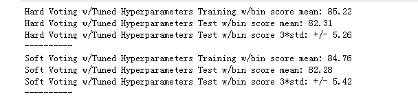
#Hard Vote or majority rules w/Tuned Hyperparameters
grid_hard = ensemble.VotingClassifier(estimators = vote_est , voting = 'hard')
grid_hard_cv = model_selection.cross_validate(grid_hard, data1[data1_x_bin], data1[Target], cv  = cv_split)
grid_hard.fit(data1[data1_x_bin], data1[Target])

print("Hard Voting w/Tuned Hyperparameters Training w/bin score mean: {:.2f}". format(grid_hard_cv['train_score'].mean()*100)) 
print("Hard Voting w/Tuned Hyperparameters Test w/bin score mean: {:.2f}". format(grid_hard_cv['test_score'].mean()*100))
print("Hard Voting w/Tuned Hyperparameters Test w/bin score 3*std: +/- {:.2f}". format(grid_hard_cv['test_score'].std()*100*3))
print('-'*10)

#Soft Vote or weighted probabilities w/Tuned Hyperparameters
grid_soft = ensemble.VotingClassifier(estimators = vote_est , voting = 'soft')
grid_soft_cv = model_selection.cross_validate(grid_soft, data1[data1_x_bin], data1[Target], cv  = cv_split)
grid_soft.fit(data1[data1_x_bin], data1[Target])

print("Soft Voting w/Tuned Hyperparameters Training w/bin score mean: {:.2f}". format(grid_soft_cv['train_score'].mean()*100)) 
print("Soft Voting w/Tuned Hyperparameters Test w/bin score mean: {:.2f}". format(grid_soft_cv['test_score'].mean()*100))
print("Soft Voting w/Tuned Hyperparameters Test w/bin score 3*std: +/- {:.2f}". format(grid_soft_cv['test_score'].std()*100*3))
print('-'*10)

 

#prepare data for modeling
print(data_val.info())
print("-"*10)
#data_val.sample(10)

 

#handmade decision tree - submission score = 0.77990
data_val['Survived'] = mytree(data_val).astype(int)

#decision tree w/full dataset modeling submission score: defaults= 0.76555, tuned= 0.77990
#submit_dt = tree.DecisionTreeClassifier()
#submit_dt = model_selection.GridSearchCV(tree.DecisionTreeClassifier(), param_grid=param_grid, scoring = 'roc_auc', cv = cv_split)
#submit_dt.fit(data1[data1_x_bin], data1[Target])
#print('Best Parameters: ', submit_dt.best_params_) #Best Parameters: {'criterion': 'gini', 'max_depth': 4, 'random_state': 0}
#data_val['Survived'] = submit_dt.predict(data_val[data1_x_bin])

#bagging w/full dataset modeling submission score: defaults= 0.75119, tuned= 0.77990
#submit_bc = ensemble.BaggingClassifier()
#submit_bc = model_selection.GridSearchCV(ensemble.BaggingClassifier(), param_grid= {'n_estimators':grid_n_estimator, 'max_samples': grid_ratio, 'oob_score': grid_bool, 'random_state': grid_seed}, scoring = 'roc_auc', cv = cv_split)
#submit_bc.fit(data1[data1_x_bin], data1[Target])
#print('Best Parameters: ', submit_bc.best_params_) #Best Parameters: {'max_samples': 0.25, 'n_estimators': 500, 'oob_score': True, 'random_state': 0}
#data_val['Survived'] = submit_bc.predict(data_val[data1_x_bin])

#extra tree w/full dataset modeling submission score: defaults= 0.76555, tuned= 0.77990
#submit_etc = ensemble.ExtraTreesClassifier()
#submit_etc = model_selection.GridSearchCV(ensemble.ExtraTreesClassifier(), param_grid={'n_estimators': grid_n_estimator, 'criterion': grid_criterion, 'max_depth': grid_max_depth, 'random_state': grid_seed}, scoring = 'roc_auc', cv = cv_split)
#submit_etc.fit(data1[data1_x_bin], data1[Target])
#print('Best Parameters: ', submit_etc.best_params_) #Best Parameters: {'criterion': 'entropy', 'max_depth': 6, 'n_estimators': 100, 'random_state': 0}
#data_val['Survived'] = submit_etc.predict(data_val[data1_x_bin])

#random foreset w/full dataset modeling submission score: defaults= 0.71291, tuned= 0.73205
#submit_rfc = ensemble.RandomForestClassifier()
#submit_rfc = model_selection.GridSearchCV(ensemble.RandomForestClassifier(), param_grid={'n_estimators': grid_n_estimator, 'criterion': grid_criterion, 'max_depth': grid_max_depth, 'random_state': grid_seed}, scoring = 'roc_auc', cv = cv_split)
#submit_rfc.fit(data1[data1_x_bin], data1[Target])
#print('Best Parameters: ', submit_rfc.best_params_) #Best Parameters: {'criterion': 'entropy', 'max_depth': 6, 'n_estimators': 100, 'random_state': 0}
#data_val['Survived'] = submit_rfc.predict(data_val[data1_x_bin])

 

#ada boosting w/full dataset modeling submission score: defaults= 0.74162, tuned= 0.75119
#submit_abc = ensemble.AdaBoostClassifier()
#submit_abc = model_selection.GridSearchCV(ensemble.AdaBoostClassifier(), param_grid={'n_estimators': grid_n_estimator, 'learning_rate': grid_ratio, 'algorithm': ['SAMME', 'SAMME.R'], 'random_state': grid_seed}, scoring = 'roc_auc', cv = cv_split)
#submit_abc.fit(data1[data1_x_bin], data1[Target])
#print('Best Parameters: ', submit_abc.best_params_) #Best Parameters: {'algorithm': 'SAMME.R', 'learning_rate': 0.1, 'n_estimators': 300, 'random_state': 0}
#data_val['Survived'] = submit_abc.predict(data_val[data1_x_bin])

#gradient boosting w/full dataset modeling submission score: defaults= 0.75119, tuned= 0.77033
#submit_gbc = ensemble.GradientBoostingClassifier()
#submit_gbc = model_selection.GridSearchCV(ensemble.GradientBoostingClassifier(), param_grid={'learning_rate': grid_ratio, 'n_estimators': grid_n_estimator, 'max_depth': grid_max_depth, 'random_state':grid_seed}, scoring = 'roc_auc', cv = cv_split)
#submit_gbc.fit(data1[data1_x_bin], data1[Target])
#print('Best Parameters: ', submit_gbc.best_params_) #Best Parameters: {'learning_rate': 0.25, 'max_depth': 2, 'n_estimators': 50, 'random_state': 0}
#data_val['Survived'] = submit_gbc.predict(data_val[data1_x_bin])

#extreme boosting w/full dataset modeling submission score: defaults= 0.73684, tuned= 0.77990
#submit_xgb = XGBClassifier()
#submit_xgb = model_selection.GridSearchCV(XGBClassifier(), param_grid= {'learning_rate': grid_learn, 'max_depth': [0,2,4,6,8,10], 'n_estimators': grid_n_estimator, 'seed': grid_seed}, scoring = 'roc_auc', cv = cv_split)
#submit_xgb.fit(data1[data1_x_bin], data1[Target])
#print('Best Parameters: ', submit_xgb.best_params_) #Best Parameters: {'learning_rate': 0.01, 'max_depth': 4, 'n_estimators': 300, 'seed': 0}
#data_val['Survived'] = submit_xgb.predict(data_val[data1_x_bin])

#hard voting classifier w/full dataset modeling submission score: defaults= 0.75598, tuned = 0.77990
#data_val['Survived'] = vote_hard.predict(data_val[data1_x_bin])
data_val['Survived'] = grid_hard.predict(data_val[data1_x_bin])

#soft voting classifier w/full dataset modeling submission score: defaults= 0.73684, tuned = 0.74162
#data_val['Survived'] = vote_soft.predict(data_val[data1_x_bin])
#data_val['Survived'] = grid_soft.predict(data_val[data1_x_bin])

#submit file
submit = data_val[['PassengerId','Survived']]
submit.to_csv("F:/wd.jupyter/datasets/kaggle_data/titanic/submit.csv", index=False)

print('Validation Data Distribution: \n', data_val['Survived'].value_counts(normalize = True))
submit.sample(10)

 

十二、步骤7：优化和制定战略
结论
　　我们的模型收敛于0.77990提交准确性。使用相同的数据集和决策树（adaboost，随机森林，梯度增强，xgboost等）的不同实现与调整不超过0.77990提交准确性。有趣的是，对此数据集，简单决策树算法具有最佳默认提交分数，并且调整获得了相同的最佳准确度分数。

虽然在单个数据集上测试少量算法无法得出一般结论，但对所提到的数据集有几个观察结果。

• 训练数据集具有与测试/验证数据集和群体不同的分布。这在交叉验证（CV）准确度分数和Kaggle提交准确度分数之间创造了广泛的差距。
• 给定相同的数据集，基于决策树的算法在适当调整后似乎收敛于相同的准确度分数。尽管进行调整，

对于迭代二，我会花更多的时间在预处理和特征工程上。为了更好地调整CV分数和Kaggle分数并提高整体准确性。