python数学工具（一）

python  数学工具包括：

1.函数的逼近

　　1.1.回归

　　1.2.插值

2.凸优化
3.积分
4.符号数学

 

本文介绍函数的逼近的回归方法

1.作为基函数的单项式

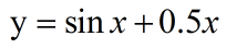
对函数 的拟合

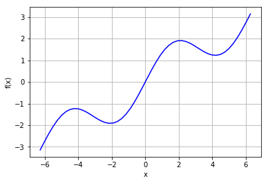
首先定义函数并且可视化

import numpy as np
import matplotlib.pyplot as plt
import pandas as pd

def f(x):
    return np.sin(x)+0.5*x

x=np.linspace(-2*np.pi,2*np.pi,50)
plt.plot(x,f(x),'b')
plt.xlabel('x')
plt.ylabel('f(x)')
plt.grid(True)

　

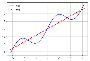
先用一次函数拟合

reg=np.polyfit(x,f(x),deg=1)
ry=np.polyval(reg,x)
plt.plot(x,f(x),'b',label='f(x)')
plt.grid(True)
plt.plot(x,ry,'r.',label='reg')
plt.legend(loc=0)

　　

 

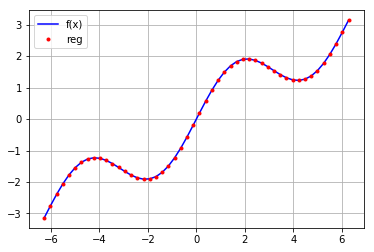
再用高次函数进行拟合

 

reg=np.polyfit(x,f(x),deg=16)
ry=np.polyval(reg,x)
plt.plot(x,f(x),'b',label='f(x)')
plt.grid(True)
plt.plot(x,ry,'r.',label='reg')
plt.legend(loc=0)

　　

拟合效果的检查

print('平均误差：',sum((ry-f(x))**2)/len(x))

平均误差： 3.16518401761e-13

　　

np.allclose(ry,f(x))

True

　

2.单独的基函数

首先常见一个空的矩阵，然后为任一行添加函数

mat=np.zeros((3+1,len(x)))
mat[3,:]=x**3
mat[2,:]=x**2
mat[1,:]=x
mat[0,:]=1

reg=np.linalg.lstsq(mat.T,f(x))

#输出系数
reg[0]

array([  1.52685368e-14,   5.62777448e-01,  -1.11022302e-15,
        -5.43553615e-03])

　　

#输出图形
ry=np.dot(reg[0],mat)


plt.plot(x,f(x),'b',label='f(x)')
plt.plot(x,ry,'r.',label='reg')
plt.grid(True)
plt.legend(loc=0)

　　

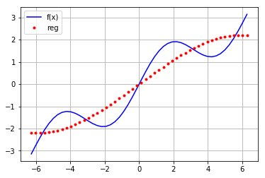
对每行的基函数进行变换：

mat=np.zeros((3+1,len(x)))
mat[3,:]=np.sin(x)
mat[2,:]=x**2
mat[1,:]=x
mat[0,:]=1

reg=np.linalg.lstsq(mat.T,f(x))

ry=np.dot(reg[0],mat)


plt.plot(x,f(x),'b',label='f(x)')
plt.plot(x,ry,'r.',label='reg')
plt.grid(True)
plt.legend(loc=0)

　　

3.多维情形

def fm(x,y):
    return np.sin(x) + 0.25 * x + np.sqrt(y) + 0.05**y*2


x = np.linspace(0, 10, 20)
y = np.linspace(0, 10, 20)
x, y = np. meshgrid( x, y)

Z = fm(x,y)
x = x.flatten()
y = x. flatten()

import statsmodels.api as sm

matrix=np.zeros((len(x),6+1))

matrix[:,6] = np.sqrt(y)
matrix[:,5] = np.sin(x)
matrix[:,4] = y**2
matrix[:,3] = y**2
matrix[:,2] = y
matrix[:,1] = x
matrix[:,0] = 1

res=sm.OLS(fm(x,y),matrix).fit()

print(res.summary().as_text())

　　

                         OLS Regression Results                            
==============================================================================
Dep. Variable:                      y   R-squared:                       0.999
Model:                            OLS   Adj. R-squared:                  0.999
Method:                 Least Squares   F-statistic:                 9.605e+04
Date:                Tue, 31 Jul 2018   Prob (F-statistic):               0.00
Time:                        10:51:36   Log-Likelihood:                 661.47
No. Observations:                 400   AIC:                            -1313.
Df Residuals:                     395   BIC:                            -1293.
Df Model:                           4                                         
Covariance Type:            nonrobust                                         
==============================================================================
                 coef    std err          t      P>|t|      [0.025      0.975]
------------------------------------------------------------------------------
const          1.9548      0.010    193.732      0.000       1.935       1.975
x1             0.5891      0.005    111.546      0.000       0.579       0.600
x2             0.5891      0.005    111.546      0.000       0.579       0.600
x3            -0.0150      0.000    -54.014      0.000      -0.016      -0.014
x4            -0.0150      0.000    -54.014      0.000      -0.016      -0.014
x5             0.9533      0.004    251.168      0.000       0.946       0.961
x6            -1.6190      0.020    -79.979      0.000      -1.659      -1.579
==============================================================================
Omnibus:                        4.352   Durbin-Watson:                   0.880
Prob(Omnibus):                  0.113   Jarque-Bera (JB):                4.214
Skew:                          -0.208   Prob(JB):                        0.122
Kurtosis:                       2.717   Cond. No.                     4.93e+17
==============================================================================