Python 画极坐标图

需要用Python画极坐标等值线图，以下是所学的一些东西，特此记录

--------------------------------------------------

翻译自 https://stackoverflow.com/questions/9071084/polar-contour-plot-in-matplotlib-best-modern-way-to-do-it

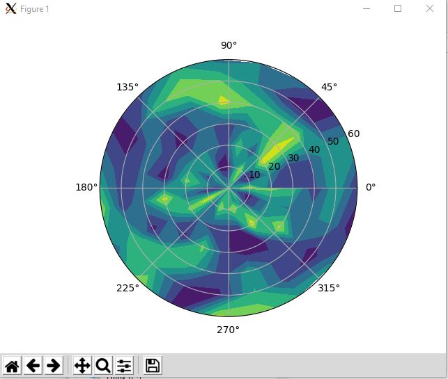
你应该能够像往常一样使用极地图的ax.contour或ax.contourf 。单位是弧度，传递函数的顺序是，theta,r

import numpy as np
import matplotlib.pyplot as plt

#-- Generate Data -----------------------------------------
# Using linspace so that the endpoint of 360 is included...
azimuths = np.radians(np.linspace(0, 360, 20))
zeniths = np.arange(0, 70, 10)

r, theta = np.meshgrid(zeniths, azimuths)
values = np.random.random((azimuths.size, zeniths.size))

#-- Plot... ------------------------------------------------
fig, ax = plt.subplots(subplot_kw=dict(projection='polar'))
ax.contourf(theta, r, values)

plt.show()

结果

 

翻译自http://blog.rtwilson.com/producing-polar-contour-plots-with-matplotlib/

创建一些极坐标轴，在上面绘制轮廓图：

fig, ax = subplots(subplot_kw=dict(projection='polar'))

cax = ax.contourf(theta, r, values, nlevels)

这个利用了contourf函数，产生了一个填充的轮廓图，使用轮廓函数可以得到简单的轮廓线。这个函数的前三个参数必须被被给定，它们都是二维数组，包含：半径raddi，角度（theta）和轮廓的实际值。最后一个参数是要绘制的轮廓的层次数——如果希望得到等值线图，则数字可以小一些，如果希望得到填充的等值线图，则数字需要大一些（以获得平滑的外观）。（如果希望最外面的轮廓足够圆，则需要网格点足够密集）

我从来没有完全理解这些二维数组，以及为什么需要它们。我通常以三个列表的形式获得我的数据，这些列表基本上是表的列，其中表的每一行都定义了一个点和值。例如：

Radius　　　Theta　　　　Value
10　　　　　　0　　　　　  0.7
10　　　　　 90　　　　　 0.45
10　　　　  180 　　     0.9
10    　　　270   　　  0.23
20　　　　   0    　　   0.5
20    　　　90    　　  0.13
20    　　 180    　　 0.52
20        270 　　    0.98

  这些行中的每一行都定义一个点 - 例如，第一行定义半径为10的点，角度为0度，值为0.7。我永远无法理解为什么轮廓功能不只是采用这三个列表并绘制一个等高线图。事实上，我已经编写了一个函数来完成这个，我将在下面描述，但首先让我解释一下这些值是如何转换为二维数组的。

首先，让我们想一想维数：我们的数据中显然有维数，半径和角度。事实上，我们可以重新塑造我们的数值数组，使得它变成二维的。我们可以从上表中看到，我们正在做半径为10度的所有方位角，然后是半径为20度的相同方位角，等等。因此，我们的值不是存储在一维列表中，我们可以把它们放在一个二维表中，其中列是方位角，行是半径：

       0      90     180    270
10    0.7    0.45    0.9    0.23
20    0.5    0.13    0.52    0.98

 这正是我们需要为contourf函数赋予的那种二维数组。这并不难理解——但为什么地球上的半径和角度数组也必须是二维的。好吧，基本上我们只需要两个像上面那样的数组，但是在对应的单元格中有相应的半径和角度，而不是值。所以，对于角度，我们有：

      0    90    180    270
10    0    90    180    270
20    0    90    180    270

对于半径，我们有：

      0    90    180   270
10    10   10    10    10
20    0    20    20    20

 

然后，当我们将所有三个数组放在一起时，每个单元格将定义我们需要的三个信息。因此，左上角的单元格给出的角度为0，半径为10，值为0.7。幸运的是，你不必手动制作这些数组——一个名为meshgrid的方便的NumPy函数会为你做：

>>> radii = np.arange(0, 60, 10)
>>> print(radii)
[ 0 10 20 30 40 50]
>>> angles = np.arange(0, 360, 90)
>>> print(angles)
[  0  90 180 270]
>>> np.meshgrid(angles, radii)
[array([[  0,  90, 180, 270],
       [  0,  90, 180, 270],
       [  0,  90, 180, 270],
       [  0,  90, 180, 270],
       [  0,  90, 180, 270],
       [  0,  90, 180, 270]]), array([[ 0,  0,  0,  0],
       [10, 10, 10, 10],
       [20, 20, 20, 20],
       [30, 30, 30, 30],
       [40, 40, 40, 40],
       [50, 50, 50, 50]])]

 要记住的一点是绘图函数需要以弧度而不是度数作为的角度（θ）的单位，因此如果您的数据是以度为单位（通常是），那么您需要使用NumPy radians函数将其转换为弧度。

完成所有这些操作后，您可以正确地将数据导入轮廓绘图功能，并且可以获得一些极轴，以便绘制它。但是，如果你这样做，你会发现你的轴看起来像这样:

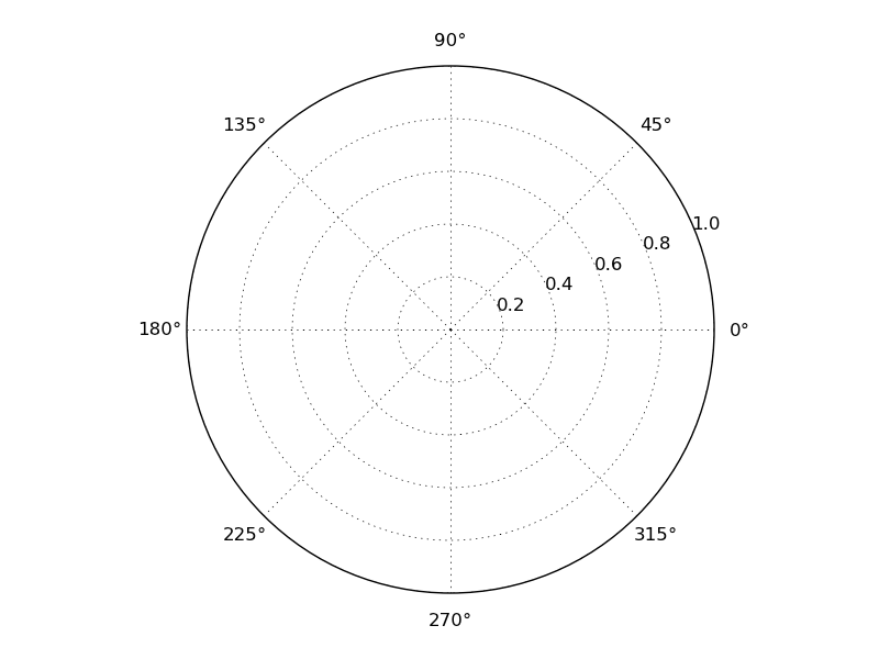
您可以看到零度不在顶部，它位于“东”或“3点”位置，并且角度绕错了方向！显然，这些事情通常都是在数学中完成的——但在我的领域，特别是人们希望有一个顶部为零像指南针一样的极坐标情景！

如果您尝试找到如何执行此操作，您将找到一个StackOverflow答案，其中包含PolarAxes的精彩子类，可以解决这个问题。很赞的是，matplotlib允许你进行这种私人定制，但是如果你看下面接受的答案，你会找到一个名为set_theta_zero_location的函数的matplotlib文档的链接。这个功能非常好地采用指南针方向（“N”或“E”或“NE”等）为零！类似地，函数set_theta_direction设置角度增加的方向。您需要做的就是从轴对象中调用它们：

ax.set_theta_zero_location("N")

ax.set_theta_direction(-1)

上面的示例将为“正常”罗盘样式绘图设置图，北部为零度，并且角度顺时针增加。如果您发现这些代码行出现错误，则需要更新matplotlib版本——这些方法仅在最新版本（v1.1.0）中添加。

所以，现在我们已经涵盖了我逐渐学到的所有这些，我们可以把它们放在一个函数中。每当我想要绘制一个极坐标等高线图时，我都会使用下面的函数，它对我来说很好。

我不能保证代码对你有用，但希望这篇文章有用，你现在可以离开并在matplotlib中创建极坐标等高线图。

import numpy as np
from matplotlib.pyplot import *
 
def plot_polar_contour(values, azimuths, zeniths):
    """Plot a polar contour plot, with 0 degrees at the North.
 
    Arguments:
 
     * `values` -- A list (or other iterable - eg. a NumPy array) of the values to plot on the
     contour plot (the `z` values)
     * `azimuths` -- A list of azimuths (in degrees)
     * `zeniths` -- A list of zeniths (that is, radii)
 
    The shapes of these lists are important, and are designed for a particular
    use case (but should be more generally useful). The values list should be `len(azimuths) * len(zeniths)`
    long with data for the first azimuth for all the zeniths, then the second azimuth for all the zeniths etc.
 
    This is designed to work nicely with data that is produced using a loop as follows:
 
    values = []
    for azimuth in azimuths:
      for zenith in zeniths:
        # Do something and get a result
        values.append(result)
 
    After that code the azimuths, zeniths and values lists will be ready to be passed into this function.
 
    """
    theta = np.radians(azimuths)
    zeniths = np.array(zeniths)
 
    values = np.array(values)
    values = values.reshape(len(azimuths), len(zeniths))
 
    r, theta = np.meshgrid(zeniths, np.radians(azimuths))
    fig, ax = subplots(subplot_kw=dict(projection='polar'))
    ax.set_theta_zero_location("N")
    ax.set_theta_direction(-1)
    autumn()
    cax = ax.contourf(theta, r, values, 30)
    autumn()
    cb = fig.colorbar(cax)
    cb.set_label("Pixel reflectance")
 
    return fig, ax, cax

 https://www.pythonprogramming.in/plot-polar-graph-in-matplotlib.html