

神经网络量化--per-channel量化
(本文首发于公众号,没事来逛逛)
之前写的关于网络量化的文章都是基于 per-layer 实现的,最近有小伙伴询问关于 per-channel 量化的问题,我发现有些同学对这个东西存在一些误解,包括我以前也被 per-channel 的字面意义误导过,所以今天简单聊一下 per-channel 量化是怎么回事。
回顾一下Per-layer量化
在介绍 per-channel 量化之前,我们先回顾一下 per-layer 量化是怎么做的。
假设 \(r_1\)、\(r_2\) 分别表示输入的 feature 和卷积的 kernel,\(r_3\) 表示输出,那么卷积运算可以表示为:
公式里面,\(oc\) 表示输出通道的 index,\(ic\) 表示输入通道的 index。下面为了公式简洁,我会省略 \(i\)、\(j\) 这些跟位置相关的 index。
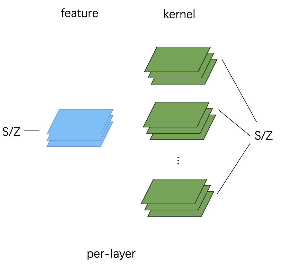
per-layer 量化下,整个 tensor 会共用一个 scale 和 zero point。
就像下面这张图给出的这样:
因此量化后的卷积运算为:
可以得出:
什么是Per-channel量化
对于 per-channel 量化来说,很多同学第一感觉就是,给 feature 和 kernel 的每一个 channel 都单独计算一个 scale 和 zeropoint,如下图所示:
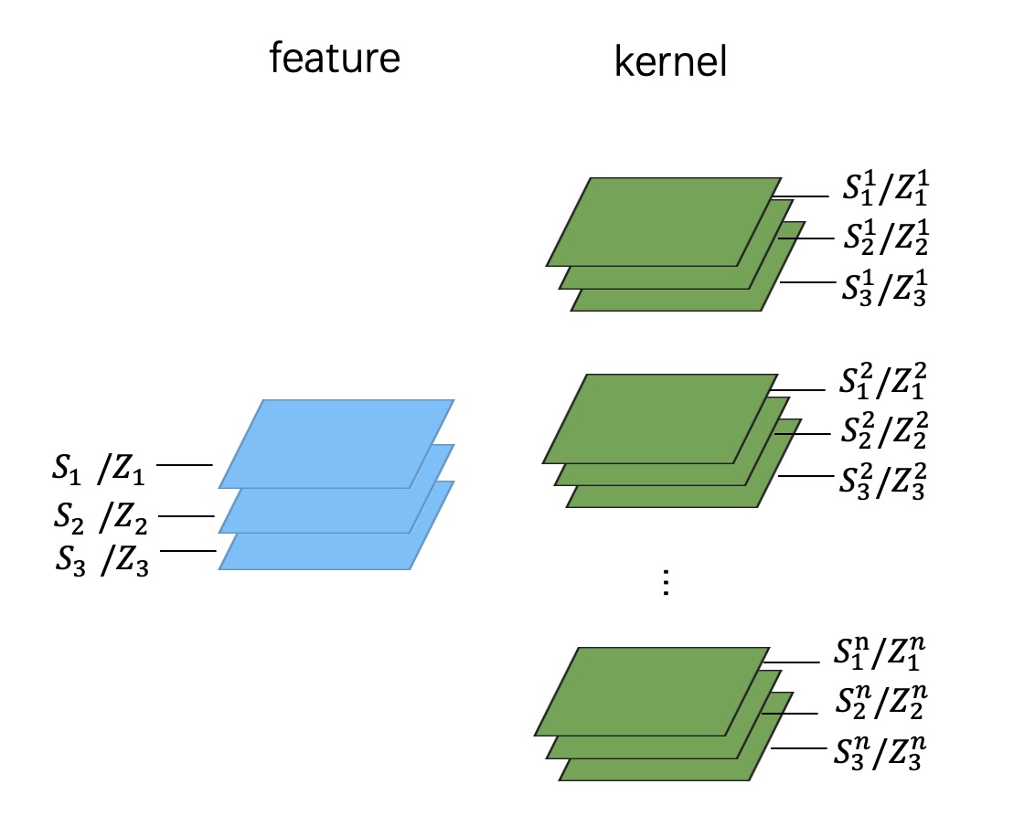
当然,从数学上看这是完全可以实现的,精度也会比较高,但在工程实现上,这种方式就行不通了。我们来看看为什么。
假设给 feature 和 kernel 的每一个 channel 都算一个 scale 和 zero point,那么公式 (2) 就变成了:
最后可以算出:
这里和前面 per-layer 最大的区别就在于,\(\frac{S_1^{ic}S_2^{ic}}{S_3}\) 这一项我们没办法在整体求和之后再做了,需要每个 input channel 计算的时候,都先用这一项 requant 一下,最后再把每个 channel 的结果相加,这样一来,卷积就没法加速了,计算开销会成倍上升。
因此,在实践中,per-channel 量化其实是按照下图的方式做的:
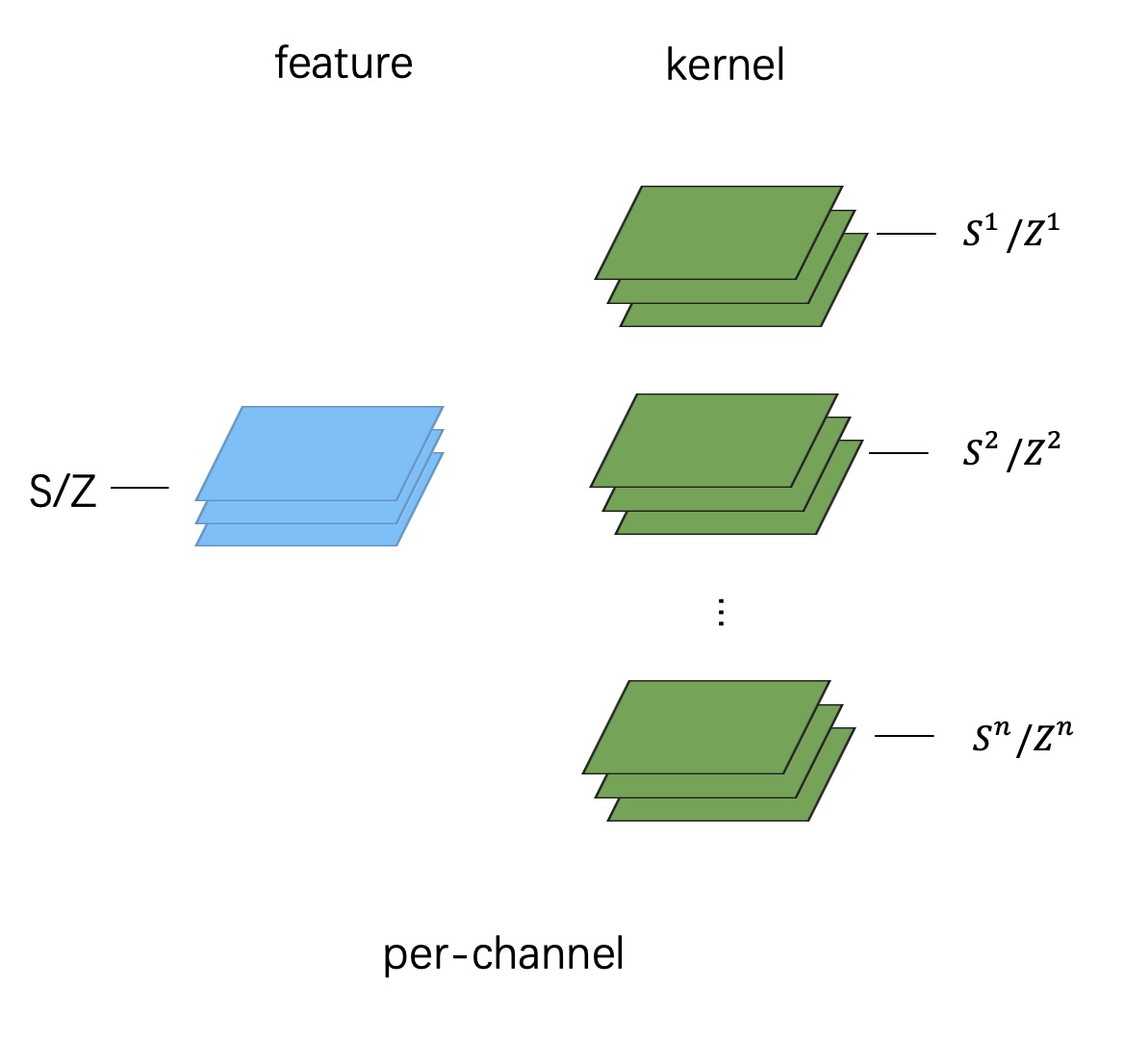
这其中的差别就在于,feature 还是整个 tensor 共用一个 scale 和 zeropoint,但每个 kernel 会单独统计一个 scale 和 zeropoint(注意是每个 kernel,而不是 kernel 的每个 channel)。
在谷歌的白皮书上,也强调了这一点:
Improved accuracy can be obtained by adapting the quantizer parameters to each kernel within the tensor....per-channel quantization has a different scale and offset for each convolutional kernel. We do not consider per-channel quantization for activations as this would complicate the inner product computations at the core of conv and matmul operations.
在这种定义下,per-channel 量化和 per-layer 就变得很相似了:
换算一下得到:
仔细对比一下前面的公式 (3),你会发现公式 (7) 和 (3) 几乎一模一样。不过,这里面的差别在于,对于不同的 \(oc\),\(q_3^{oc}\) 对应的 \(S_2\) 是不一样的,因为每个 kernel 都会有自己专属的 \(S_2\)。因此,对于每一个 \(oc\),需要单独用 \(\frac{S_1S_2}{S_3}\) 重新 requant 一下。而在 per-layer 量化里面,我们是可以把整个 output feature 都算完,再统一 requant 的。
工程实现
由于 pytorch 的限制,我没法在 python 层面模拟 per-channel 量化,只能做一下量化训练时的 fake quantize,而这一步并不难,因此,我们还是直接看一下一些底层推理库是怎么实现的。
这里以 NCNN 和 tflite 为例。
NCNN
首先看 NCNN 相关的实现。其实 NCNN 的量化方式本身就是 per-channel 实现的。下面这段代码片段分别是 NCNN 对 kernel 和 feature 的量化操作(感谢知乎@田子宸的解读)
// ========= 量化kernel =========
for (int n=0; n<num_output; n++)    // 每个kernel单独量化
{
  Layer* op = ncnn::create_layer(ncnn::LayerType::Quantize);

  ncnn::ParamDict pd;
  pd.set(0, weight_data_int8_scales[n]);// 设置scale参数

  op->load_param(pd);

  op->create_pipeline(opt_cpu);

  ncnn::Option opt;
  opt.blob_allocator = int8_weight_data.allocator;
  // 拆开计算后组合
  const Mat weight_data_n = weight_data.range(weight_data_size_output * n, weight_data_size_output);
  Mat int8_weight_data_n = int8_weight_data.range(weight_data_size_output * n, weight_data_size_output);
  op->forward(weight_data_n, int8_weight_data_n, opt);    // 计算量化值

  delete op;
}

weight_data = int8_weight_data; // 替代原来的weight_data


// =========== 量化输入feature ============

// initial the quantize,dequantize op layer
// 初始化输入/输出的量化/反量化Op
if (use_int8_inference)
{
  // 创建量化Op,不run
  quantize = ncnn::create_layer(ncnn::LayerType::Quantize);
  {
    ncnn::ParamDict pd;
    pd.set(0, bottom_blob_int8_scale);// 所有输入用同一个scale

    quantize->load_param(pd);

    quantize->create_pipeline(opt_cpu);
  }

  // 创建反量化Op,不Run
  dequantize_ops.resize(num_output);  // 由于不同kernel weight的scale是不同的
  for (int n=0; n<num_output; n++)    // 因此反量化scale也是不同的
  {
    dequantize_ops[n] = ncnn::create_layer(ncnn::LayerType::Dequantize);

    float top_rescale = 1.f;

    if (weight_data_int8_scales[n] == 0)
      top_rescale = 0;
    else    // 反量化scale=1/(输入scale*权重scale),即一个反映射
      top_rescale = 1.f / (bottom_blob_int8_scale * weight_data_int8_scales[n]);

    dequantize_ops[n]->load_param(pd);

    // 省略若干代码
    ....

    dequantize_scales.push_back(top_rescale);
  }
}

quantize->forward(bottom_blob, bottom_blob_int8, opt_g);    // 量化计算
可以看到,对 kernel 的量化会针对每个 kernel 设置 scale,而对输入的 feature 则是用同一个 scale 进行量化。
此外,在 dequantize 这一步则是每个 channel 也会设置一个 requant(反量化)的 scale,这个 scale 对应的数值是 \(\frac{1}{S_1S_2}\)。前面说了,per-channel 里面每个 kernel 的 \(S_2\) 都是不一样的,所以这里需要对每个 channel 进行反量化。
从代码里面也可以看出,NCNN 采用的是对称量化的方式(因为没有用到 zero point),并且在量化运算结束后,会将得到的 int32 数值 requant 回 float32,并不是全量化的方式。所以在 dequantize 这一步其实对应的是公式(6),而非公式(7)。
tflite
每次看 tflite 的代码都感觉不适,从这个角度讲,NCNN 算是一个很了不起的框架了,代码结构整齐划一,模块分得很清晰,非常适合小白入门学习。而 tflite 的代码由于做了大量优化,而且整个项目的模块划分很混乱,所以你甚至不知道要从哪个地方开始阅读。
下面这段代码是我从 tflite 中截取的一段(链接:https://github.com/tensorflow/tensorflow/blob/v1.15.0/tensorflow/lite/kernels/internal/reference/conv.h#L101)
inline void Conv(const ConvParams& params, const RuntimeShape& input_shape,
                 const uint8* input_data, const RuntimeShape& filter_shape,
                 const uint8* filter_data, const RuntimeShape& bias_shape,
                 const int32* bias_data, const RuntimeShape& output_shape,
                 uint8* output_data, const RuntimeShape& im2col_shape,
                 uint8* im2col_data, void* cpu_backend_context) {
  // 省略若干代码
  ....

  for (int batch = 0; batch < batches; ++batch) {
    for (int out_y = 0; out_y < output_height; ++out_y) {
      for (int out_x = 0; out_x < output_width; ++out_x) {
        // 单独计算每个output channel
        for (int out_channel = 0; out_channel < output_depth; ++out_channel) {
          const int in_x_origin = (out_x * stride_width) - pad_width;
          const int in_y_origin = (out_y * stride_height) - pad_height;
          int32 acc = 0;
          for (int filter_y = 0; filter_y < filter_height; ++filter_y) {
            for (int filter_x = 0; filter_x < filter_width; ++filter_x) {
              for (int in_channel = 0; in_channel < input_depth; ++in_channel) {
                const int in_x = in_x_origin + dilation_width_factor * filter_x;
                const int in_y =
                    in_y_origin + dilation_height_factor * filter_y;
                // If the location is outside the bounds of the input image,
                // use zero as a default value.
                if ((in_x >= 0) && (in_x < input_width) && (in_y >= 0) &&
                    (in_y < input_height)) {
                  int32 input_val = input_data[Offset(input_shape, batch, in_y,
                                                      in_x, in_channel)];
                  int32 filter_val =
                      filter_data[Offset(filter_shape, out_channel, filter_y,
                                         filter_x, in_channel)];
                  acc +=
                      (filter_val + filter_offset) * (input_val + input_offset);
                }
              }
            }
          }
          if (bias_data) {
            acc += bias_data[out_channel];
          }

          // 每个channel算完都做一次requant,
          // 这里采用fixed multiplier + bitshift的形式,不需要反量化回fp32
          acc = MultiplyByQuantizedMultiplier(acc, output_multiplier,
                                              output_shift);
          acc += output_offset;
          acc = std::max(acc, output_activation_min);
          acc = std::min(acc, output_activation_max);
          output_data[Offset(output_shape, batch, out_y, out_x, out_channel)] =
              static_cast<uint8>(acc);
        }
      }
    }
  }
}
从这里可以看出,tflite 采用的也是 per-channel 量化的方式(至少 1.5 这个版本是这样)。不过相比 NCNN 有一点优化是不需要反量化回 float,而是直接通过 fixed multiplier+bitshift 的形式直接算出下一步的输入,对应公式 (7)。
总结
这篇文章介绍了 per-channel 量化的过程,以及这么做的缘由。简单概括就是,per-channel 量化是对每个 kernel 计算不同的量化参数,其余的和 per-layer 没有区别。这么做最主要是出于计算性能的考虑。从这里我们又再次看到,模型量化是和底层实现紧密结合的技术。
参考
- https://zhuanlan.zhihu.com/p/71881443
- Quantizing deep convolutional networks for efficient inference: A whitepaper
- https://github.com/tensorflow/tensorflow/blob/v1.15.0/tensorflow/lite/kernels/internal/reference/conv.h#L101
欢迎关注我的公众号:大白话AI,立志用大白话讲懂AI。

 浙公网安备 33010602011771号