论文阅读 | AMP-Net

AMP-Net

UESTC TIP 2021

Introduction

1. 再次提到 “structureinducing regularizers” (结构诱导的正则化项) 如某些变换域的稀疏性、低秩等。
2. 再次提到压缩感知重建是求解一个欠定的线性逆系统 (under-determined linear inverse system)
3. NN-based methods. “no good interpretation and theoretical guarantee”
4. deep unfolding. “a good balance between reconstruction speed and interpretation”
5. It has been proved that combining multiple kinds of image prior knowledge can get better reconstruction results than single one. 最终的工作都落在使用 DNN 建模正则项以集成更多的先验信息。
6. “data-driven end-to-end”

一些经典的非线性迭代算法，用于求解上述优化问题，包括

1. fast iterative shrinkage-thresholding algorithm (ISTA) 迭代收缩阈值算法
2. approximate message passing (AMP) 近似消息传递
3. sparse Bayesian learning
4. orthogonal matching pursuit (OMP) 正交匹配追踪
5. iterative hard thresholding (IHT)

Preliminary

优化目标由下式给出

\[\min_x \mathcal{R}(\textbf{x}), \quad \textbf{s.t. y} = \textbf{Ax} \tag{1} \]

\(\mathcal{R}(\textbf{x})\) 为正则项。约束 \(\textbf{y}=\textbf{Ax}\) 的含义是，由于问题是欠定的 (数次提到 \(M \ll N\))，满足这个约束的重建有很多种。而正则项 \(\mathcal{R}(\cdot)\) 正是用于进行结构先验的约束 (类似 Inpainting 中利用正则项进行风格约束)

AMP Algorithm

The AMP algorithm interprets the classical linear operation as the sum of the original data and a noise term:

\[\textbf{A}^T(\textbf{y}-\textbf{Ax}')+\textbf{x}' \tag{2} \]

where \(\textbf{x}' \in \mathbb{R}^N\) is an estimate of \(\textbf{x}\). (前面看起来是 \(\frac{1}{2}\|\textbf{Ax}'-\textbf{y}\|_2^2\) 的梯度更新方向，整体就是 \(\textbf{x}'\) 的更新)

Backgrounds

AMP 分析了迭代非线性算法的一个经典方案

\[\begin{aligned} \textbf{z}^{k-1}&=\textbf{y}-\textbf{Ax}^{k-1} \\ \tag{3} \textbf{x}^k &= \mathcal{T}_k (\textbf{A}^T \textbf{z}^{k-1} + \textbf{x}^{k-1}) \end{aligned}\]

式中

• \(\textbf{A}\): 采样矩阵
• \(\mathcal{T}_k(\cdot)\): 非线性函数

这里求 \(\textbf{z}^{k-1}\) 并计算 \((\textbf{A}^T \textbf{z}^{k-1} + \textbf{x}^{k-1})\) 与 ISTA-Net 求 \(\textbf{r}^{(k)}\) 实际上做的是同一件事，第二步也是差不多的，都是在梯度更新后的 \(\textbf{x}'\) 上再进行一次非线性操作 (即此处的 \(\mathcal{T}_k\))，即：保真 (约束) 项和正则项交替计算。

这里 AMP 把 \(\textbf{x}^{k-1} \rightarrow \textbf{x}^{k}\) 过程解释为 \(\bar{\textbf{x}}+\textbf{e}\)，后者是一个 Gaussian Noise. AMP 把迭代过程解释为 去噪视角 (denoising perspective).

是否可以由此引入 Diffusion

Architecture

Overview

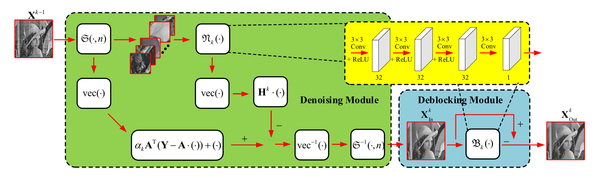
整体结构如图所示。

Sampling Model

ISTA-Net 没有详细讲述采样过程 (其采样矩阵是固定的)，但 AMP-Net 是一个端到端网络，并进行了精讲。

\[\mathbf{Y} = \mathbf{A} \ \text{vec}(\mathcal{S}(\mathbf{X}, n)) \tag{4} \]

式中 \(\mathbf{X}\in\mathbb{R}^{L \times P}\) 为原始输入的单通道图像，\(\mathbf{Y}\in\mathbb{R}^{M \times I}\) 为采样后的测量值。\(\mathbf{A}\) 是可学习的。从整个网络的顶层视角来看，\(\mathbf{X}\) 是网络的输入，输出 \(\mathbf{X}'\) ，像是训练了一个自编码器。

Reconstruction Model

由 Initialization Module 和 Reconstruction Module 组成。首先，Initialization Module 生成一个合理的初始化估计。后有多个 Reconstruction Module，又由 Denoising Module 和 Deblocking Module 组成。

Reconstruction Module 完成的任务如下。

\[\mathbf{X}^0 = \mathcal{S}^{-1}\left(\text{vec}^{-1}(\mathbf{B}\mathbf{Y}), n\right) \tag{5} \]

注意 \(\textbf{X}^0\) 与 \(\textbf{X}\) 不同，是我们从 \(\textbf{Y}\) 重建出来的。

\(\mathbf{B}\) 是可学习的。区别于 ISTA-Net 直接用 \(\mathbf{X}\) 的先验对 \(\mathbf{X}^0\) 初始化

\[\begin{aligned} \mathbf{Q}_{\text{init}} &= \arg\min_{\mathbf{Q}} \|\mathbf{Q}\mathbf{Y} - \mathbf{X}\|_F^2 = \mathbf{X}\mathbf{Y}^\top (\mathbf{Y}\mathbf{Y}^\top)^{-1} \\ \tag{6} \mathbf{x}^{(0)}&=\mathbf{Q}_{init}\textbf{y} \end{aligned}\]

观察 ASP-Net 的更新过程

\[\mathbf{x}_k^i = \alpha_k \mathbf{A}^\top \mathbf{z}_{k-1}^i + \mathbf{x}_{k-1}^i - (\alpha_k \mathbf{A}^\top \mathbf{A} - \mathbf{I}) \text{vec}(\mathcal{N}_k(\mathbf{X}_{k-1}^i)) \tag{7} \]

前两项是梯度下降。之后需要过一次非线性变换 (对应前文 \(\min_x \mathcal{R}(\textbf{x})\) 形式)，这里是把 \(\mathcal{N}_k\) 用神经网络建模了。最后得到的是一个加性的非线性变换，可表述为 (省略了 \(\textbf{x}_i\) 经 \(\mathcal{S}^{-1}(\cdot, \textbf{x})\) 替换为 \(\mathbf{X}_i\) 的过程)

\[\mathbf{X}^k = \mathbf{X}^{k-1} - \mathcal{D}^k(\mathbf{X}^{k-1}) \tag{8} \]

这里 \(\mathcal{D}(\cdot)\) 可以代表一个非线性的去噪过程，因为 AMP 把迭代过程中含 \(\bar{x}_i - x_{k-1}\) 的项视为一个噪声。区别于 ISTA-Net，其过程表述为

\[\mathbf{X}^k = \mathcal{D}^k(\mathbf{X}^{k-1}) \tag{9} \]

接下来是 Deblocking Module.

“Reconstructing images block-by-block without overlapping may lead to a situation that additional deblocking operations must be carried out.”

这里也是 ASP-Net 一直在强调的 block-by-block，即 \(\mathcal{S}(\cdot)\) 的主要任务。提到，这个操作可能需要一步额外的去噪，因而再次应用 denoising perspective 思想，即

\[\mathbf{X}^k=\bar{\mathbf{X}}+\mathbf{E} \tag{10} \]

从而

\[\mathbf{X}_k^{\text{Out}} = \mathbf{X}_k^{\text{In}} - \mathcal{B}_k(\mathbf{X}_k^{\text{In}}) \tag{11} \]

\(\mathcal{B}_k\) 也使用网络来建模。

(所以一开始为什么要进行分块)

Loss

只有一个 \(\ell_2\).

Experiments

比 ISTA-Net 效果更好，可能原因

1. 采样过程也纳入可学习的范畴，从 \(\mathbf{X}\) 提取到更充分的先验
2. 网络层数更多 (?)