论文阅读 | ISTA-Net

ISTA-Net

KAUST CVPR’18

Introduction

1. 利用信号固有的冗余性，CS 策略可以边采样边压缩，相较于传统 JPEG 技术等“先采样后压缩”策略，节省带宽和存储空间
2. CS 证明，只要信号在某些变换域中表现出 稀疏性 (sparsity)，则可以用比 Nyquist 采样定理更少的不等距采样来高概率地重建信号。
3. 传统方法利用一些 结构化稀疏 (structured sparsity) 作为图像先验，然后以迭代的方式求解 稀疏正则化 (sparsity-regularized) 优化问题。
4. 该工作将用于一般 \(\ell_1\)-norm CS 重建模型的 ISTA 映射到一个深度网络中。
5. 该工作使用了非线性、可学习的稀疏变换，和开发了一种高效的策略解决非线性变换的 近端映射 (proixmal mapping)。☞
6. ISTA-Nets 可认为是两种 CS 方法 (optimization-based 与 non-iterative algorithms，即 network-based) 之间的桥梁

Preliminary

CS Reconstruction

\[\begin{aligned} &\text{Infer: } \text{x} \in \mathbb{R}^N \\ \tag{1} &\text{From: }\text{y} = \Phi \text{x} \in\mathbb{R}^M\text{ where }M\ll N \end{aligned}\]

其中

• \(\text{x}\): original signal
• \(\text{y}\): randomized CS measurements
• \(\Phi\in\mathbb{R}^{M \times N}\): linear random projection
• define CS ratio as \(\frac{M}{N}\)

从 CS 测量域到原始信号域的逆映射问题是欠定的 (ill-posed)，即解不稳定或不唯一。

Related Work

讨论两类 (optimization-based 与 non-iterative algorithms) 压缩感知重建方法。

Optimization-based

Given:

\[\text{linear measurements \textbf{y}} \]

Reconstruct the original image \(\textbf{x}\) by solving the following optimization problem:

\[\min_x \frac{1}{2} \|\Phi \textbf{x} - \textbf{y}\|_2^2 + \lambda \|\Psi \textbf{x}\|_1 \tag{2} \]

向量 \(\Psi \textbf{x}\) 解释是表示 \(\textbf{x}\) 关于某个变换 \(\Psi\) 的 变换系数 (transform coefficients)，比如通过 \(\ell_1\)-norm 用于约束稀疏性，\(\lambda\) 为正则化系数。后面这一项是正则项，除促进稀疏性外，避免过拟合。

由于自然图像是 非平稳 (non-stationary) 的，经典的 固定域方法 (DCT, 小波, 梯度域) 性能不佳。许多工作将关于变换系数的额外的先验纳入 CS 重建框架中。

存在的问题

1. 迭代次数多，计算复杂性
2. 依赖先验

Network-based

…

Methodology

Traditional ISTA

“The iterative shrinkage-thresholding algorithm (ISTA) is a popular first order proximal method, which is well suited for solving many large-scale linear inverse problems.”

迭代收缩 (软) 阈值算法 (ISTA) 是一种一阶近似方法，非常适合求解许多大型线性反问题。

最终 ISTA 是要解决一个近端映射问题

\[\text{prox}_{\lambda\phi}(\textbf{r}) \tag{3} \]

提到，由于 \(\Psi\) 可能是非正交 (如果是矩阵) 乃至非线性的，\(\text{prox}\) 的计算成本很高。且受限于 \(\rho\) 和 \(\lambda\) 等超参 (非参数化 ??) 的手动设置。

ISTA-Net

思路是把 ISTA 的每一轮迭代 (steps) 映射到一个 DNN 的 phases，当然这样一来 steps 是固定的。

有点像，Attention 一次性处理了 RNN 中串行处理的向量序列。

整体架构如下图所示。

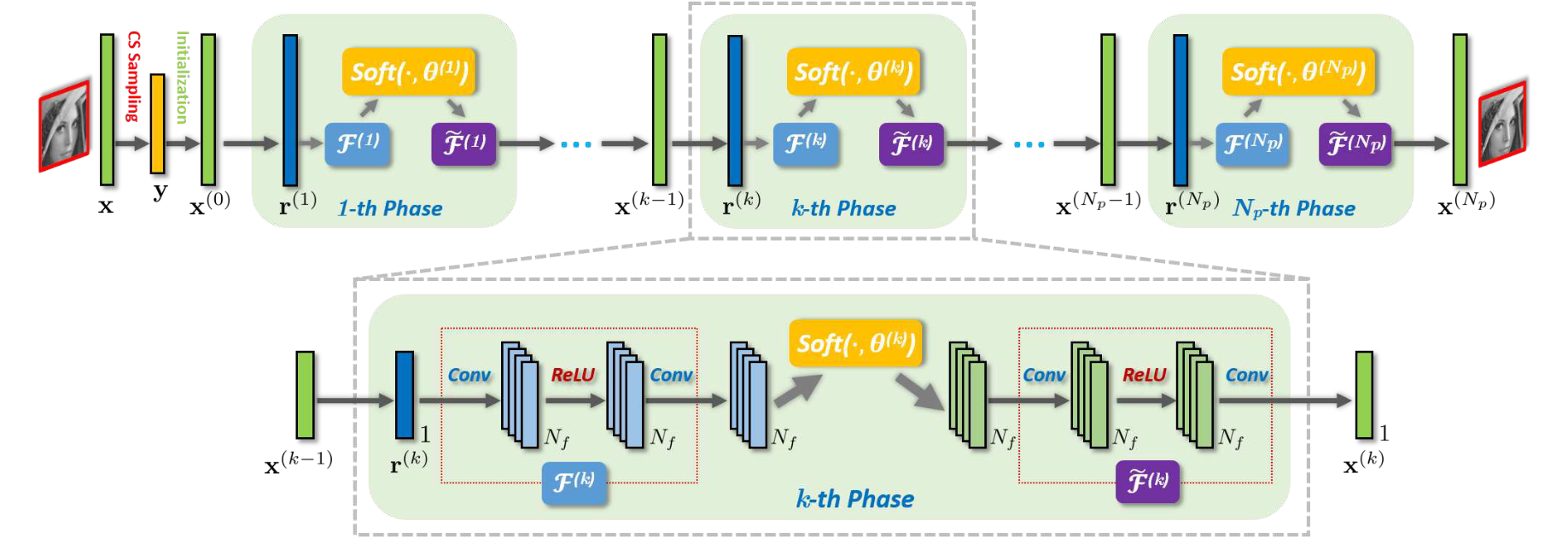
ISTA-Net 将手动设置的 \(\Psi\) 建模为一个参数化的非线性变换，记为 \(\mathcal{F}(\cdot)\)，实现为

\[\begin{aligned} &\mathcal{F}(\textbf{x}) = \textbf{B}ReLU(\textbf{Ax}) \\ \tag{4} &\text{Conv3×3 → ReLU → Conv3×3} \end{aligned}\]

卷积层 \(N_f\) 个通道，对应 \(N_f\) 次滤波。学习率 \(\rho\) 在 phases 间可变。

Assumption In the context of image inverse problems, one general and reasonable assumption is that each element of \((x^{(k)} − r^{(k)})\) follows an independent normal distribution with common zero mean and variance \(\sigma^2\).

在使用网络对正则项建模的过程中还提到一个 \(soft\) 函数，这个 \(soft\) 是 软阈值函数，由原文 Eq. (9) 求导得到。

\[\mathcal{F}(\textbf{x}^{(k)})=soft(\mathcal{F}(\textbf{r}^{(k)}), \theta) \tag{5} \]

引入 \(\mathcal{F}\) 的左逆 \(\tilde{\mathcal{F}}\)，即 \(\mathcal{F}\circ\tilde{\mathcal{F}}=\mathcal{I}\)

\[\textbf{x}^{(k)}=\tilde{\mathcal{F}}(soft(\mathcal{F}(\textbf{r}^{(k)}), \theta)) \tag{6} \]

这个逆运算的成立由损失函数进行约束。

Initialization

使用线性映射而非随机初始化。

\[Q_{\text{init}} = \arg \min_{Q} \| QY - X \|_F^2 = XY^{\top} (YY^{\top})^{-1} \tag{7} \]

从而 \(\forall{\textbf{y}},\textbf{x}^{(0)}=\textbf{Q}_{init}\textbf{y}\)

损失函数由 \(\ell_2\) 和 \(\mathcal{L}_{constraint}\) 组成。约束形式为

\[\tilde{\mathcal{F}}(\mathcal{F}(\textbf{x}_i))-\textbf{x}_i \tag{8} \]

注意 Compressive Sensing 是 Inverse Problem，其训练数据对格式为 \(\{(\textbf{y}_i, \textbf{x}_i)\}\).

ISTA-Net+

使用更深的网络进行建模。

Assume that

\[\textbf{x}^{(k)} = \textbf{r}^{(k)} + \textbf{w}^{(k)} + \textbf{e}^{(k)} \tag{9} \]

其中

• \(\textbf{w}^{(k)}\): 补充高频
• \(\textbf{e}^{(k)}\): 噪声

(看完 ASP-Net 再回来看，引入 \(\mathcal{G}\) 补充高频与 ASP-Net 引入 \(\mathcal{B}\) 进行 deblocking 是否是类似的，都可视为某种去噪过程呢)

Summary

代码写得非常清晰，不再赘述。

思考，这个模型是不是压缩感知重建的标准模板。即

\[n \text{ iterations} \times\{\text{GD}→\text{non-linear}(\textbf{x}^{k-1})→\text{denoising}→\textbf{x}^k\} \]