Pytorch的主要组成模块

一、基本配置

对于一个PyTorch项目，我们需要导入一些Python常用的包来帮助我们快速实现功能。常见的包有os、numpy等，此外还需要调用PyTorch自身一些模块便于灵活使用，比如torch、torch.nn、torch.utils.data.Dataset、torch.utils.data.DataLoader、torch.optimizer等等。

首先导入必须的包。注意这里只是建议导入的包导入的方式，可以采用不同的方案，比如涉及到表格信息的读入很可能用到pandas，对于不同的项目可能还需要导入一些更上层的包如cv2等。如果涉及可视化还会用到matplotlib、seaborn等。涉及到下游分析和指标计算也常用到sklearn。

import os
import numpy as np
import torch
import torch.nn as nn
from torch.utils.data import Dataset, DataLoader
import torch.optim as optimizer

根据前面我们对深度学习任务的梳理，有如下几个超参数可以统一设置，方便后续调试时修改：

batch size
初始学习率（初始）
训练次数（max_epochs）
GPU配置

batch_size = 16
# 批次的大小
lr = 1e-4
# 优化器的学习率
max_epochs = 100

GPU的设置有两种常见的方式：

# 方案一：使用os.environ，这种情况如果使用GPU不需要设置
os.environ['CUDA_VISIBLE_DEVICES'] = '0,1'

# 方案二：使用“device”，后续对要使用GPU的变量用.to(device)即可
device = torch.device("cuda:1" if torch.cuda.is_available() else "cpu")

当然还会有一些其他模块或用户自定义模块会用到的参数，有需要也可以在一开始进行设置。

二、数据读入

PyTorch数据读入是通过Dataset+DataLoader的方式完成的，Dataset定义好数据的格式和数据变换形式，DataLoader用iterative的方式不断读入批次数据。

我们可以定义自己的Dataset类来实现灵活的数据读取，定义的类需要继承PyTorch自身的Dataset类。主要包含三个函数：

__init__: 用于向类中传入外部参数，同时定义样本集
__getitem__: 用于逐个读取样本集合中的元素，可以进行一定的变换，并将返回训练/验证所需的数据
__len__: 用于返回数据集的样本数

下面以cifar10数据集为例给出构建Dataset类的方式：

import torch
from torchvision import datasets
train_data = datasets.ImageFolder(train_path, transform=data_transform)
val_data = datasets.ImageFolder(val_path, transform=data_transform)

这里使用了PyTorch自带的ImageFolder类的用于读取按一定结构存储的图片数据（path对应图片存放的目录，目录下包含若干子目录，每个子目录对应属于同一个类的图片）。

其中“data_transform”可以对图像进行一定的变换，如翻转、裁剪等操作，可自己定义。这里我们会在下一章通过实战加以介绍。

这里另外给出一个例子，其中图片存放在一个文件夹，另外有一个csv文件给出了图片名称对应的标签。

class MyDataset(Dataset):
    def __init__(self, data_dir, info_csv, image_list, transform=None):
        """
        Args:
            data_dir: path to image directory.
            info_csv: path to the csv file containing image indexes
                with corresponding labels.
            image_list: path to the txt file contains image names to training/validation set
            transform: optional transform to be applied on a sample.
        """
        label_info = pd.read_csv(info_csv)
        image_file = open(image_list).readlines()
        self.data_dir = data_dir
        self.image_file = image_file
        self.label_info = label_info
        self.transform = transform

    def __getitem__(self, index):
        """
        Args:
            index: the index of item
        Returns:
            image and its labels
        """
        image_name = self.image_file[index].strip('\n')
        raw_label = self.label_info.loc[self.label_info['Image_index'] == image_name]
        label = raw_label.iloc[:,0]
        image_name = os.path.join(self.data_dir, image_name)
        image = Image.open(image_name).convert('RGB')
        if self.transform is not None:
            image = self.transform(image)
        return image, label

    def __len__(self):
        return len(self.image_file)

构建好Dataset后，就可以使用DataLoader来按批次读入数据了，实现代码如下：

from torch.utils.data import DataLoader

train_loader = torch.utils.data.DataLoader(train_data, batch_size=batch_size, num_workers=4, shuffle=True, drop_last=True)
val_loader = torch.utils.data.DataLoader(val_data, batch_size=batch_size, num_workers=4, shuffle=False)

其中:

batch_size：样本是按“批”读入的，batch_size就是每次读入的样本数
num_workers：有多少个进程用于读取数据
shuffle：是否将读入的数据打乱
drop_last：对于样本最后一部分没有达到批次数的样本，使其不再参与训练

这里可以看一下我们的加载的数据。PyTorch中的DataLoader的读取可以使用next和iter来完成

import matplotlib.pyplot as plt
images, labels = next(iter(val_loader))
print(images.shape)
plt.imshow(images[0].transpose(1,2,0))
plt.show()

三、模型构建

人工智能的第三次浪潮受益于卷积神经网络的出现和BP反向传播算法的实现，随着深度学习的发展，研究人员研究出了许许多多的模型，PyTorch中神经网络构造一般是基于 Module 类的模型来完成的，它让模型构造更加灵活。

3.1 神经网络的构造

Module 类是 nn 模块里提供的一个模型构造类，是所有神经⽹网络模块的基类，我们可以继承它来定义我们想要的模型。下面继承 Module 类构造多层感知机。这里定义的 MLP 类重载了 Module 类的 init 函数和 forward 函数。它们分别用于创建模型参数和定义前向计算。前向计算也即正向传播。

import torch
from torch import nn

class MLP(nn.Module):
  # 声明带有模型参数的层，这里声明了两个全连接层
  def __init__(self, **kwargs):
    # 调用MLP父类Block的构造函数来进行必要的初始化。这样在构造实例时还可以指定其他函数
    super(MLP, self).__init__(**kwargs)
    self.hidden = nn.Linear(784, 256)
    self.act = nn.ReLU()
    self.output = nn.Linear(256,10)
    
   # 定义模型的前向计算，即如何根据输入x计算返回所需要的模型输出
  def forward(self, x):
    o = self.act(self.hidden(x))
    return self.output(o)

以上的 MLP 类中⽆须定义反向传播函数。系统将通过⾃动求梯度⽽自动⽣成反向传播所需的 backward 函数。

我们可以实例化 MLP 类得到模型变量 net 。下⾯的代码初始化 net 并传入输⼊数据 X 做一次前向计算。其中， net(X) 会调用 MLP 继承⾃自 Module 类的 call 函数，这个函数将调⽤用 MLP 类定义的forward 函数来完成前向计算。

X = torch.rand(2,784)
net = MLP()
print(net)
net(X)

输出：
MLP(
(hidden): Linear(in_features=784, out_features=256, bias=True)
(act): ReLU()
(output): Linear(in_features=256, out_features=10, bias=True)
)
tensor([[ 0.0149, -0.2641, -0.0040, 0.0945, -0.1277, -0.0092, 0.0343, 0.0627,
-0.1742, 0.1866],
[ 0.0738, -0.1409, 0.0790, 0.0597, -0.1572, 0.0479, -0.0519, 0.0211,
-0.1435, 0.1958]], grad_fn=)

注意，这里并没有将 Module 类命名为 Layer (层)或者 Model (模型)之类的名字，这是因为该类是一个可供⾃由组建的部件。它的子类既可以是⼀个层(如PyTorch提供的 Linear 类)，⼜可以是一个模型(如这里定义的 MLP 类)，或者是模型的⼀个部分。

3.2 神经网络中常见的层

深度学习的一个魅力在于神经网络中各式各样的层，例如全连接层、卷积层、池化层与循环层等等。虽然PyTorch提供了⼤量常用的层，但有时候我们依然希望⾃定义层。使用 Module 来自定义层，可以被反复调用。

不含模型参数的层
含模型参数的层
二维卷积层
池化层

3.2.1 不含模型参数的层

先介绍如何定义一个不含模型参数的自定义层。下⾯构造的 MyLayer 类通过继承 Module 类自定义了一个将输入减掉均值后输出的层，并将层的计算定义在了 forward 函数里。这个层里不含模型参数。

import torch
from torch import nn

class MyLayer(nn.Module):
    def __init__(self, **kwargs):
        super(MyLayer, self).__init__(**kwargs)
    def forward(self, x):
        return x - x.mean()

测试，实例化该层，然后做前向计算

layer = MyLayer()
layer(torch.tensor([1, 2, 3, 4, 5], dtype=torch.float))

tensor([-2., -1.,  0.,  1.,  2.])

3.2.2 含模型参数的层

还可以自定义含模型参数的自定义层。其中的模型参数可以通过训练学出。

Parameter 类其实是 Tensor 的子类，如果一个 Tensor 是 Parameter ，那么它会⾃动被添加到模型的参数列表里。所以在⾃定义含模型参数的层时，我们应该将参数定义成 Parameter ，除了直接定义成 Parameter 类外，还可以使⽤ ParameterList 和 ParameterDict 分别定义参数的列表和字典。

class MyListDense(nn.Module):
    def __init__(self):
        super(MyListDense, self).__init__()
        self.params = nn.ParameterList([nn.Parameter(torch.randn(4, 4)) for i in range(3)])
        self.params.append(nn.Parameter(torch.randn(4, 1)))

    def forward(self, x):
        for i in range(len(self.params)):
            x = torch.mm(x, self.params[i])
        return x
net = MyListDense()
print(net)

class MyDictDense(nn.Module):
    def __init__(self):
        super(MyDictDense, self).__init__()
        self.params = nn.ParameterDict({
                'linear1': nn.Parameter(torch.randn(4, 4)),
                'linear2': nn.Parameter(torch.randn(4, 1))
        })
        self.params.update({'linear3': nn.Parameter(torch.randn(4, 2))}) # 新增

    def forward(self, x, choice='linear1'):
        return torch.mm(x, self.params[choice])

net = MyDictDense()
print(net)

下面给出常见的神经网络的一些层，比如卷积层、池化层，以及较为基础的AlexNet，LeNet等。

3.2.3 二维卷积层

二维卷积层将输入和卷积核做互相关运算，并加上一个标量偏差来得到输出。卷积层的模型参数包括了卷积核和标量偏差。在训练模型的时候，通常我们先对卷积核随机初始化，然后不断迭代卷积核和偏差。

import torch
from torch import nn

# 卷积运算（二维互相关）
def corr2d(X, K): 
    h, w = K.shape
    X, K = X.float(), K.float()
    Y = torch.zeros((X.shape[0] - h + 1, X.shape[1] - w + 1))
    for i in range(Y.shape[0]):
        for j in range(Y.shape[1]):
            Y[i, j] = (X[i: i + h, j: j + w] * K).sum()
    return Y

# 二维卷积层
class Conv2D(nn.Module):
    def __init__(self, kernel_size):
        super(Conv2D, self).__init__()
        self.weight = nn.Parameter(torch.randn(kernel_size))
        self.bias = nn.Parameter(torch.randn(1))

    def forward(self, x):
        return corr2d(x, self.weight) + self.bias

卷积窗口形状为 p×q 的卷积层称为 p×q 卷积层。同样， p×q 卷积或 p×q 卷积核说明卷积核的高和宽分别为 p 和 q。

填充(padding)是指在输⼊高和宽的两侧填充元素(通常是0元素)。

下面的例子里我们创建一个⾼和宽为3的二维卷积层，然后设输⼊高和宽两侧的填充数分别为1。给定一个高和宽为8的输入，我们发现输出的高和宽也是8。

import torch
from torch import nn

# 定义一个函数来计算卷积层。它对输入和输出做相应的升维和降维
import torch
from torch import nn

# 定义一个函数来计算卷积层。它对输入和输出做相应的升维和降维
def comp_conv2d(conv2d, X):
    # (1, 1)代表批量大小和通道数
    X = X.view((1, 1) + X.shape)
    Y = conv2d(X)
    return Y.view(Y.shape[2:]) # 排除不关心的前两维:批量和通道


# 注意这里是两侧分别填充1⾏或列，所以在两侧一共填充2⾏或列
conv2d = nn.Conv2d(in_channels=1, out_channels=1, kernel_size=3,padding=1)

X = torch.rand(8, 8)
comp_conv2d(conv2d, X).shape

输出：
torch.Size([8, 8])

当卷积核的高和宽不同时，我们也可以通过设置高和宽上不同的填充数使输出和输入具有相同的高和宽。

# 使用高为5、宽为3的卷积核。在⾼和宽两侧的填充数分别为2和1
conv2d = nn.Conv2d(in_channels=1, out_channels=1, kernel_size=(5, 3), padding=(2, 1))
comp_conv2d(conv2d, X).shape

输出：
torch.Size([8, 8])

在二维互相关运算中，卷积窗口从输入数组的最左上方开始，按从左往右、从上往下的顺序，依次在输⼊数组上滑动。我们将每次滑动的行数和列数称为步幅(stride)。

conv2d = nn.Conv2d(1, 1, kernel_size=(3, 5), padding=(0, 1), stride=(3, 4))
comp_conv2d(conv2d, X).shape

输出：
torch.Size([2, 2])

填充可以增加输出的高和宽。这常用来使输出与输入具有相同的高和宽。
步幅可以减小输出的高和宽，例如输出的高和宽仅为输入的高和宽的 ( 为大于1的整数)。

3.2.4 池化层

池化层每次对输入数据的一个固定形状窗口(⼜称池化窗口)中的元素计算输出。不同于卷积层里计算输⼊和核的互相关性，池化层直接计算池化窗口内元素的最大值或者平均值。该运算也分别叫做最大池化或平均池化。在二维最⼤池化中，池化窗口从输入数组的最左上方开始，按从左往右、从上往下的顺序，依次在输⼊数组上滑动。当池化窗口滑动到某⼀位置时，窗口中的输入子数组的最大值即输出数组中相应位置的元素。

下面把池化层的前向计算实现在pool2d函数里。

import torch
from torch import nn

def pool2d(X, pool_size, mode='max'):
    p_h, p_w = pool_size
    Y = torch.zeros((X.shape[0] - p_h + 1, X.shape[1] - p_w + 1))
    for i in range(Y.shape[0]):
        for j in range(Y.shape[1]):
            if mode == 'max':
                Y[i, j] = X[i: i + p_h, j: j + p_w].max()
            elif mode == 'avg':
                Y[i, j] = X[i: i + p_h, j: j + p_w].mean()
    return Y

X = torch.tensor([[0, 1, 2], [3, 4, 5], [6, 7, 8]], dtype=torch.float)
pool2d(X, (2, 2))

输出：
tensor([[4., 5.],
[7., 8.]])

pool2d(X, (2, 2), 'avg')

输出：
tensor([[2., 3.],
[5., 6.]])

可以使用torch.nn包来构建神经网络。nn包则依赖于autograd包来定义模型并对它们求导。一个nn.Module包含各个层和一个forward(input)方法，该方法返回output。

3.3 模型示例

3.3.1 LeNet

这是一个简单的前馈神经网络 (feed-forward network）（LeNet）。它接受一个输入，然后将它送入下一层，一层接一层的传递，最后给出输出。

一个神经网络的典型训练过程如下：

1. 定义包含一些可学习参数(或者叫权重）的神经网络
1. 在输入数据集上迭代
1. 通过网络处理输入
1. 计算 loss (输出和正确答案的距离）
1. 将梯度反向传播给网络的参数
1. 更新网络的权重，一般使用一个简单的规则：weight = weight - learning_rate * gradient

import torch
import torch.nn as nn
import torch.nn.functional as F


class Net(nn.Module):

    def __init__(self):
        super(Net, self).__init__()
        # 输入图像channel：1；输出channel：6；5x5卷积核
        self.conv1 = nn.Conv2d(1, 6, 5)
        self.conv2 = nn.Conv2d(6, 16, 5)
        # an affine operation: y = Wx + b
        self.fc1 = nn.Linear(16 * 5 * 5, 120)
        self.fc2 = nn.Linear(120, 84)
        self.fc3 = nn.Linear(84, 10)

    def forward(self, x):
        # 2x2 Max pooling
        x = F.max_pool2d(F.relu(self.conv1(x)), (2, 2))
        # 如果是方阵,则可以只使用一个数字进行定义
        x = F.max_pool2d(F.relu(self.conv2(x)), 2)
        x = x.view(-1, self.num_flat_features(x))
        x = F.relu(self.fc1(x))
        x = F.relu(self.fc2(x))
        x = self.fc3(x)
        return x

    def num_flat_features(self, x):
        size = x.size()[1:]  # 除去批处理维度的其他所有维度
        num_features = 1
        for s in size:
            num_features *= s
        return num_features


net = Net()
print(net)

Net(
(conv1): Conv2d(1, 6, kernel_size=(5, 5), stride=(1, 1))
(conv2): Conv2d(6, 16, kernel_size=(5, 5), stride=(1, 1))
(fc1): Linear(in_features=400, out_features=120, bias=True)
(fc2): Linear(in_features=120, out_features=84, bias=True)
(fc3): Linear(in_features=84, out_features=10, bias=True)
)

我们只需要定义 forward 函数，backward函数会在使用autograd时自动定义，backward函数用来计算导数。我们可以在 forward 函数中使用任何针对张量的操作和计算。

一个模型的可学习参数可以通过net.parameters()返回

params = list(net.parameters())
print(len(params))
print(params[0].size())  # conv1的权重

输出:
10
torch.Size([6, 1, 5, 5])

让我们尝试一个随机的 32x32 的输入。注意:这个网络 (LeNet）的期待输入是 32x32 的张量。如果使用 MNIST 数据集来训练这个网络，要把图片大小重新调整到 32x32。

input = torch.randn(1, 1, 32, 32)
out = net(input)
print(out)

清零所有参数的梯度缓存，然后进行随机梯度的反向传播：

net.zero_grad()
out.backward(torch.randn(1, 10))

注意：torch.nn只支持小批量处理 (mini-batches）。整个 torch.nn 包只支持小批量样本的输入，不支持单个样本的输入。比如，nn.Conv2d 接受一个4维的张量，即nSamples x nChannels x Height x Width 如果是一个单独的样本，只需要使用input.unsqueeze(0) 来添加一个“假的”批大小维度。

torch.Tensor - 一个多维数组，支持诸如backward()等的自动求导操作，同时也保存了张量的梯度。
nn.Module - 神经网络模块。是一种方便封装参数的方式，具有将参数移动到GPU、导出、加载等功能。
nn.Parameter - 张量的一种，当它作为一个属性分配给一个Module时，它会被自动注册为一个参数。
autograd.Function - 实现了自动求导前向和反向传播的定义，每个Tensor至少创建一个Function节点，该节点连接到创建Tensor的函数并对其历史进行编码。

3.3.2 AlexNet

下面再介绍一个比较基础的案例AlexNet

class AlexNet(nn.Module):
    def __init__(self):
        super(AlexNet, self).__init__()
        self.conv = nn.Sequential(
            nn.Conv2d(1, 96, 11, 4), # in_channels, out_channels, kernel_size, stride, padding
            nn.ReLU(),
            nn.MaxPool2d(3, 2), # kernel_size, stride
            # 减小卷积窗口，使用填充为2来使得输入与输出的高和宽一致，且增大输出通道数
            nn.Conv2d(96, 256, 5, 1, 2),
            nn.ReLU(),
            nn.MaxPool2d(3, 2),
            # 连续3个卷积层，且使用更小的卷积窗口。除了最后的卷积层外，进一步增大了输出通道数。
            # 前两个卷积层后不使用池化层来减小输入的高和宽
            nn.Conv2d(256, 384, 3, 1, 1),
            nn.ReLU(),
            nn.Conv2d(384, 384, 3, 1, 1),
            nn.ReLU(),
            nn.Conv2d(384, 256, 3, 1, 1),
            nn.ReLU(),
            nn.MaxPool2d(3, 2)
        )
         # 这里全连接层的输出个数比LeNet中的大数倍。使用丢弃层来缓解过拟合
        self.fc = nn.Sequential(
            nn.Linear(256*5*5, 4096),
            nn.ReLU(),
            nn.Dropout(0.5),
            nn.Linear(4096, 4096),
            nn.ReLU(),
            nn.Dropout(0.5),
            # 输出层。由于这里使用Fashion-MNIST，所以用类别数为10，而非论文中的1000
            nn.Linear(4096, 10),
        )

    def forward(self, img):
        feature = self.conv(img)
        output = self.fc(feature.view(img.shape[0], -1))
        return output

net = AlexNet()
print(net)

AlexNet(
(conv): Sequential(
(0): Conv2d(1, 96, kernel_size=(11, 11), stride=(4, 4))
(1): ReLU()
(2): MaxPool2d(kernel_size=3, stride=2, padding=0, dilation=1, ceil_mode=False)
(3): Conv2d(96, 256, kernel_size=(5, 5), stride=(1, 1), padding=(2, 2))
(4): ReLU()
(5): MaxPool2d(kernel_size=3, stride=2, padding=0, dilation=1, ceil_mode=False)
(6): Conv2d(256, 384, kernel_size=(3, 3), stride=(1, 1), padding=(1, 1))
(7): ReLU()
(8): Conv2d(384, 384, kernel_size=(3, 3), stride=(1, 1), padding=(1, 1))
(9): ReLU()
(10): Conv2d(384, 256, kernel_size=(3, 3), stride=(1, 1), padding=(1, 1))
(11): ReLU()
(12): MaxPool2d(kernel_size=3, stride=2, padding=0, dilation=1, ceil_mode=False)
)
(fc): Sequential(
(0): Linear(in_features=6400, out_features=4096, bias=True)
(1): ReLU()
(2): Dropout(p=0.5)
(3): Linear(in_features=4096, out_features=4096, bias=True)
(4): ReLU()
(5): Dropout(p=0.5)
(6): Linear(in_features=4096, out_features=10, bias=True)
)
)

四、模型初始化

在深度学习模型的训练中，权重的初始值极为重要。一个好的权重值，会使模型收敛速度提高，使模型准确率更精确。为了利于训练和减少收敛时间，我们需要对模型进行合理的初始化。PyTorch也在torch.nn.init中为我们提供了常用的初始化方法。

4.1 torch.nn.init内容

通过访问torch.nn.init的官方文档链接，我们发现torch.nn.init提供了以下初始化方法：

1 . torch.nn.init.uniform_(tensor, a=0.0, b=1.0)
2 . torch.nn.init.normal_(tensor, mean=0.0, std=1.0)
3 . torch.nn.init.constant_(tensor, val)
4 . torch.nn.init.ones_(tensor)
5 . torch.nn.init.zeros_(tensor)
6 . torch.nn.init.eye_(tensor)
7 . torch.nn.init.dirac_(tensor, groups=1)
8 . torch.nn.init.xavier_uniform_(tensor, gain=1.0)
9 . torch.nn.init.xavier_normal_(tensor, gain=1.0)
10 . torch.nn.init.kaiming_uniform_(tensor, a=0,mode='fan__in', nonlinearity='leaky_relu')
11 . torch.nn.init.kaiming_normal_(tensor, a=0, mode='fan_in', nonlinearity='leaky_relu')
12 . torch.nn.init.orthogonal_(tensor, gain=1)
13 . torch.nn.init.sparse_(tensor, sparsity, std=0.01)
14 . torch.nn.init.calculate_gain(nonlinearity, param=None)

关于计算增益如下表：

nonlinearity	gain
Linear/Identity	1
Conv{1,2,3}D	1
Sigmod	1
Tanh	5/3
ReLU	$\sqrt{(2)}$
Leaky Relu	$\sqrt{(2/1+neg_slop^2)}$

我们可以发现这些函数除了calculate_gain，所有函数的后缀都带有下划线，意味着这些函数将会直接原地更改输入张量的值。

4.2 torch.nn.init使用

我们通常会根据实际模型来使用torch.nn.init进行初始化，通常使用isinstance来进行判断模块（回顾3.4模型构建）属于什么类型。

import torch
import torch.nn as nn

conv = nn.Conv2d(1,3,3)
linear = nn.Linear(10,1)

isinstance(conv,nn.Conv2d)
isinstance(linear,nn.Conv2d)

True
False

对于不同的类型层，我们就可以设置不同的权值初始化的方法。

# 查看随机初始化的conv参数
conv.weight.data
# 查看linear的参数
linear.weight.data

tensor([[[[ 0.1174, 0.1071, 0.2977],
[-0.2634, -0.0583, -0.2465],
[ 0.1726, -0.0452, -0.2354]]],
[[[ 0.1382, 0.1853, -0.1515],
[ 0.0561, 0.2798, -0.2488],
[-0.1288, 0.0031, 0.2826]]],
[[[ 0.2655, 0.2566, -0.1276],
[ 0.1905, -0.1308, 0.2933],
[ 0.0557, -0.1880, 0.0669]]]])

tensor([[-0.0089, 0.1186, 0.1213, -0.2569, 0.1381, 0.3125, 0.1118, -0.0063, -0.2330, 0.1956]])

# 对conv进行kaiming初始化
torch.nn.init.kaiming_normal_(conv.weight.data)
conv.weight.data
# 对linear进行常数初始化
torch.nn.init.constant_(linear.weight.data,0.3)
linear.weight.data

tensor([[[[ 0.3249, -0.0500, 0.6703],
[-0.3561, 0.0946, 0.4380],
[-0.9426, 0.9116, 0.4374]]],
[[[ 0.6727, 0.9885, 0.1635],
[ 0.7218, -1.2841, -0.2970],
[-0.9128, -0.1134, -0.3846]]],
[[[ 0.2018, 0.4668, -0.0937],
[-0.2701, -0.3073, 0.6686],
[-0.3269, -0.0094, 0.3246]]]])
tensor([[0.3000, 0.3000, 0.3000, 0.3000, 0.3000, 0.3000, 0.3000, 0.3000, 0.3000,0.3000]])

4.3 初始化函数的封装

人们常常将各种初始化方法定义为一个initialize_weights()的函数并在模型初始后进行使用。

def initialize_weights(self):
	for m in self.modules():
		# 判断是否属于Conv2d
		if isinstance(m, nn.Conv2d):
			torch.nn.init.xavier_normal_(m.weight.data)
			# 判断是否有偏置
			if m.bias is not None:
				torch.nn.init.constant_(m.bias.data,0.3)
		elif isinstance(m, nn.Linear):
			torch.nn.init.normal_(m.weight.data, 0.1)
			if m.bias is not None:
				torch.nn.init.zeros_(m.bias.data)
		elif isinstance(m, nn.BatchNorm2d):
			m.weight.data.fill_(1) 		 
			m.bias.data.zeros_()

这段代码流程是遍历当前模型的每一层，然后判断各层属于什么类型，然后根据不同类型层，设定不同的权值初始化方法。

我们可以通过下面的例程进行一个简短的演示：

# 模型的定义
class MLP(nn.Module):
  # 声明带有模型参数的层，这里声明了两个全连接层
  def __init__(self, **kwargs):
    # 调用MLP父类Block的构造函数来进行必要的初始化。这样在构造实例时还可以指定其他函数
    super(MLP, self).__init__(**kwargs)
    self.hidden = nn.Conv2d(1,1,3)
    self.act = nn.ReLU()
    self.output = nn.Linear(10,1)
    
   # 定义模型的前向计算，即如何根据输入x计算返回所需要的模型输出
  def forward(self, x):
    o = self.act(self.hidden(x))
    return self.output(o)

mlp = MLP()
print(list(mlp.parameters()))
print("-------初始化-------")

initialize_weights(mlp)
print(list(mlp.parameters()))

[Parameter containing:
tensor([[[[ 0.2103, -0.1679, 0.1757],
[-0.0647, -0.0136, -0.0410],
[ 0.1371, -0.1738, -0.0850]]]], requires_grad=True), Parameter containing:
tensor([0.2507], requires_grad=True), Parameter containing:
tensor([[ 0.2790, -0.1247, 0.2762, 0.1149, -0.2121, -0.3022, -0.1859, 0.2983,
-0.0757, -0.2868]], requires_grad=True), Parameter containing:
tensor([-0.0905], requires_grad=True)]
"-------初始化-------"
[Parameter containing:
tensor([[[[-0.3196, -0.0204, -0.5784],
[ 0.2660, 0.2242, -0.4198],
[-0.0952, 0.6033, -0.8108]]]], requires_grad=True),
Parameter containing:
tensor([0.3000], requires_grad=True),
Parameter containing:
tensor([[ 0.7542, 0.5796, 2.2963, -0.1814, -0.9627, 1.9044, 0.4763, 1.2077,
0.8583, 1.9494]], requires_grad=True),
Parameter containing:
tensor([0.], requires_grad=True)]

五、损失函数

在深度学习广为使用的今天，我们可以在脑海里清晰的知道，一个模型想要达到很好的效果需要学习，也就是我们常说的训练。一个好的训练离不开优质的负反馈，这里的损失函数就是模型的负反馈。

所以在PyTorch中，损失函数是必不可少的。它是数据输入到模型当中，产生的结果与真实标签的评价指标，我们的模型可以按照损失函数的目标来做出改进。

下面我们将开始探索pytorch的所拥有的损失函数。这里将列出PyTorch中常用的损失函数（一般通过torch.nn调用），并详细介绍每个损失函数的功能介绍、数学公式和调用代码。当然，PyTorch的损失函数还远不止这些，在解决实际问题的过程中需要进一步探索、借鉴现有工作，或者设计自己的损失函数。

5.1 二分类交叉熵损失函数

torch.nn.BCELoss(weight=None, size_average=None, reduce=None, reduction='mean')

功能：计算二分类任务时的交叉熵（Cross Entropy）函数。在二分类中，label是{0,1}。对于进入交叉熵函数的input为概率分布的形式。一般来说，input为sigmoid激活层的输出，或者softmax的输出。

主要参数：

weight:每个类别的loss设置权值

size_average:数据为bool，为True时，返回的loss为平均值；为False时，返回的各样本的loss之和。

reduce:数据类型为bool，为True时，loss的返回是标量。

计算公式如下：
$ \ell(x, y)=\left\{\begin{array}{ll} \operatorname{mean}(L), & \text { if reduction }=\text { 'mean' } \\ \operatorname{sum}(L), & \text { if reduction }=\text { 'sum' } \end{array}\right. $

m = nn.Sigmoid()
loss = nn.BCELoss()
input = torch.randn(3, requires_grad=True)
target = torch.empty(3).random_(2)
output = loss(m(input), target)
output.backward()

print('BCELoss损失函数的计算结果为',output)

BCELoss损失函数的计算结果为 tensor(0.5732, grad_fn=<BinaryCrossEntropyBackward>)

5.2 交叉熵损失函数

torch.nn.CrossEntropyLoss(weight=None, size_average=None, ignore_index=-100, reduce=None, reduction='mean')

功能：计算交叉熵函数

主要参数：

weight:每个类别的loss设置权值。

size_average:数据为bool，为True时，返回的loss为平均值；为False时，返回的各样本的loss之和。

ignore_index:忽略某个类的损失函数。

reduce:数据类型为bool，为True时，loss的返回是标量。

计算公式如下：
$ \operatorname{loss}(x, \text { class })=-\log \left(\frac{\exp (x[\text { class }])}{\sum_{j} \exp (x[j])}\right)=-x[\text { class }]+\log \left(\sum_{j} \exp (x[j])\right) $

loss = nn.CrossEntropyLoss()
input = torch.randn(3, 5, requires_grad=True)
target = torch.empty(3, dtype=torch.long).random_(5)
output = loss(input, target)
output.backward()

print(output)

tensor(2.0115, grad_fn=<NllLossBackward>)

5.3 L1损失函数

torch.nn.L1Loss(size_average=None, reduce=None, reduction='mean')

功能： 计算输出y和真实标签target之间的差值的绝对值。

我们需要知道的是，reduction参数决定了计算模式。有三种计算模式可选：none：逐个元素计算。
sum：所有元素求和，返回标量。
mean：加权平均，返回标量。
如果选择none，那么返回的结果是和输入元素相同尺寸的。默认计算方式是求平均。

计算公式如下：
$ L_{n} = |x_{n}-y_{n}| $

loss = nn.L1Loss()
input = torch.randn(3, 5, requires_grad=True)
target = torch.randn(3, 5)
output = loss(input, target)
output.backward()

print('L1损失函数的计算结果为',output)

L1损失函数的计算结果为 tensor(1.5729, grad_fn=<L1LossBackward>)

5.4 MSE损失函数

torch.nn.MSELoss(size_average=None, reduce=None, reduction='mean')

功能： 计算输出y和真实标签target之差的平方。

和L1Loss一样，MSELoss损失函数中，reduction参数决定了计算模式。有三种计算模式可选：none：逐个元素计算。
sum：所有元素求和，返回标量。默认计算方式是求平均。

计算公式如下：

$ l_{n}=\left(x_{n}-y_{n}\right)^{2} $

loss = nn.MSELoss()
input = torch.randn(3, 5, requires_grad=True)
target = torch.randn(3, 5)
output = loss(input, target)
output.backward()

print('MSE损失函数的计算结果为',output)

MSE损失函数的计算结果为 tensor(1.6968, grad_fn=<MseLossBackward>)

5.5 平滑L1 (Smooth L1)损失函数

torch.nn.SmoothL1Loss(size_average=None, reduce=None, reduction='mean', beta=1.0)

功能： L1的平滑输出，其功能是减轻离群点带来的影响

reduction参数决定了计算模式。有三种计算模式可选：none：逐个元素计算。
sum：所有元素求和，返回标量。默认计算方式是求平均。

提醒： 之后的损失函数中，关于reduction 这个参数依旧会存在。所以，之后就不再单独说明。

计算公式如下：
$ \operatorname{loss}(x, y)=\frac{1}{n} \sum_{i=1}^{n} z_{i} $
其中，
$ z_{i}=\left\{\begin{array}{ll} 0.5\left(x_{i}-y_{i}\right)^{2}, & \text { if }\left|x_{i}-y_{i}\right|<1 \\ \left|x_{i}-y_{i}\right|-0.5, & \text { otherwise } \end{array}\right. $

loss = nn.SmoothL1Loss()
input = torch.randn(3, 5, requires_grad=True)
target = torch.randn(3, 5)
output = loss(input, target)
output.backward()

print('SmoothL1Loss损失函数的计算结果为',output)

SmoothL1Loss损失函数的计算结果为 tensor(0.7808, grad_fn=<SmoothL1LossBackward>)

平滑L1与L1的对比

这里我们通过可视化两种损失函数曲线来对比平滑L1和L1两种损失函数的区别。

inputs = torch.linspace(-10, 10, steps=5000)
target = torch.zeros_like(inputs)

loss_f_smooth = nn.SmoothL1Loss(reduction='none')
loss_smooth = loss_f_smooth(inputs, target)
loss_f_l1 = nn.L1Loss(reduction='none')
loss_l1 = loss_f_l1(inputs,target)

plt.plot(inputs.numpy(), loss_smooth.numpy(), label='Smooth L1 Loss')
plt.plot(inputs.numpy(), loss_l1, label='L1 loss')
plt.xlabel('x_i - y_i')
plt.ylabel('loss value')
plt.legend()
plt.grid()
plt.show()

png

可以看出，对于smoothL1来说，在 0 这个尖端处，过渡更为平滑。

5.6 目标泊松分布的负对数似然损失

torch.nn.PoissonNLLLoss(log_input=True, full=False, size_average=None, eps=1e-08, reduce=None, reduction='mean')

功能： 泊松分布的负对数似然损失函数

主要参数：

log_input：输入是否为对数形式，决定计算公式。

full：计算所有 loss，默认为 False。

eps：修正项，避免 input 为 0 时，log(input) 为 nan 的情况。

数学公式：

当参数log_input=True：
$ \operatorname{loss}\left(x_{n}, y_{n}\right)=e^{x_{n}}-x_{n} \cdot y_{n} $
当参数log_input=False：

$
\operatorname{loss}\left(x_{n}, y_{n}\right)=x_{n}-y_{n} \cdot \log \left(x_{n}+\text { eps }\right)
$

loss = nn.PoissonNLLLoss()
log_input = torch.randn(5, 2, requires_grad=True)
target = torch.randn(5, 2)
output = loss(log_input, target)
output.backward()

print('PoissonNLLLoss损失函数的计算结果为',output)

PoissonNLLLoss损失函数的计算结果为 tensor(0.7358, grad_fn=<MeanBackward0>)

5.7 KL散度

torch.nn.KLDivLoss(size_average=None, reduce=None, reduction='mean', log_target=False)

功能： 计算KL散度，也就是计算相对熵。用于连续分布的距离度量，并且对离散采用的连续输出空间分布进行回归通常很有用。

主要参数:

reduction：计算模式，可为 none/sum/mean/batchmean。

none：逐个元素计算。

sum：所有元素求和，返回标量。

mean：加权平均，返回标量。

batchmean：batchsize 维度求平均值。

计算公式：

$ \begin{aligned} D_{\mathrm{KL}}(P, Q)=\mathrm{E}_{X \sim P}\left[\log \frac{P(X)}{Q(X)}\right] &=\mathrm{E}_{X \sim P}[\log P(X)-\log Q(X)] \\ &=\sum_{i=1}^{n} P\left(x_{i}\right)\left(\log P\left(x_{i}\right)-\log Q\left(x_{i}\right)\right) \end{aligned} $

inputs = torch.tensor([[0.5, 0.3, 0.2], [0.2, 0.3, 0.5]])
target = torch.tensor([[0.9, 0.05, 0.05], [0.1, 0.7, 0.2]], dtype=torch.float)
loss = nn.KLDivLoss()
output = loss(inputs,target)

print('KLDivLoss损失函数的计算结果为',output)

KLDivLoss损失函数的计算结果为 tensor(-0.3335)

5.8 MarginRankingLoss

torch.nn.MarginRankingLoss(margin=0.0, size_average=None, reduce=None, reduction='mean')

功能： 计算两个向量之间的相似度，用于排序任务。该方法用于计算两组数据之间的差异。

主要参数:

margin：边界值，$x_{1}$ 与$x_{2}$ 之间的差异值。

reduction：计算模式，可为 none/sum/mean。

计算公式：

$ \operatorname{loss}(x 1, x 2, y)=\max (0,-y *(x 1-x 2)+\operatorname{margin}) $

loss = nn.MarginRankingLoss()
input1 = torch.randn(3, requires_grad=True)
input2 = torch.randn(3, requires_grad=True)
target = torch.randn(3).sign()
output = loss(input1, input2, target)
output.backward()

print('MarginRankingLoss损失函数的计算结果为',output)

MarginRankingLoss损失函数的计算结果为 tensor(0.7740, grad_fn=<MeanBackward0>)

5.9 多标签边界损失函数

torch.nn.MultiLabelMarginLoss(size_average=None, reduce=None, reduction='mean')

功能： 对于多标签分类问题计算损失函数。

主要参数:

reduction：计算模式，可为 none/sum/mean。

计算公式：
$ \operatorname{loss}(x, y)=\sum_{i j} \frac{\max (0,1-x[y[j]]-x[i])}{x \cdot \operatorname{size}(0)} $

$ \begin{array}{l} \text { 其中, } i=0, \ldots, x \cdot \operatorname{size}(0), j=0, \ldots, y \cdot \operatorname{size}(0), \text { 对于所有的 } i \text { 和 } j \text {, 都有 } y[j] \geq 0 \text { 并且 }\\ i \neq y[j] \end{array} $

loss = nn.MultiLabelMarginLoss()
x = torch.FloatTensor([[0.9, 0.2, 0.4, 0.8]])
# for target y, only consider labels 3 and 0, not after label -1
y = torch.LongTensor([[3, 0, -1, 1]])# 真实的分类是，第3类和第0类
output = loss(x, y)

print('MultiLabelMarginLoss损失函数的计算结果为',output)

MultiLabelMarginLoss损失函数的计算结果为 tensor(0.4500)

5.10 二分类损失函数

torch.nn.SoftMarginLoss(size_average=None, reduce=None, reduction='mean')torch.nn.(size_average=None, reduce=None, reduction='mean')

功能： 计算二分类的 logistic 损失。

主要参数:

reduction：计算模式，可为 none/sum/mean。

计算公式：

$ \operatorname{loss}(x, y)=\sum_{i} \frac{\log (1+\exp (-y[i] \cdot x[i]))}{x \cdot \operatorname{nelement}()} $

$ \ \text { 其中, } x . \text { nelement() 为输入 } x \text { 中的样本个数。注意这里 } y \text { 也有 } 1 \text { 和 }-1 \text { 两种模式。 } \ $

inputs = torch.tensor([[0.3, 0.7], [0.5, 0.5]])  # 两个样本，两个神经元
target = torch.tensor([[-1, 1], [1, -1]], dtype=torch.float)  # 该 loss 为逐个神经元计算，需要为每个神经元单独设置标签

loss_f = nn.SoftMarginLoss()
output = loss_f(inputs, target)

print('SoftMarginLoss损失函数的计算结果为',output)

SoftMarginLoss损失函数的计算结果为 tensor(0.6764)

5.11 多分类的折页损失

torch.nn.MultiMarginLoss(p=1, margin=1.0, weight=None, size_average=None, reduce=None, reduction='mean')

功能： 计算多分类的折页损失

主要参数:

reduction：计算模式，可为 none/sum/mean。

p：可选 1 或 2。

weight：各类别的 loss 设置权值。

margin：边界值

计算公式：

$ \operatorname{loss}(x, y)=\frac{\sum_{i} \max (0, \operatorname{margin}-x[y]+x[i])^{p}}{x \cdot \operatorname{size}(0)} $

$ \begin{array}{l} \text { 其中, } x \in\{0, \ldots, x \cdot \operatorname{size}(0)-1\}, y \in\{0, \ldots, y \cdot \operatorname{size}(0)-1\} \text {, 并且对于所有的 } i \text { 和 } j \text {, }\\ \text { 都有 } 0 \leq y[j] \leq x \cdot \operatorname{size}(0)-1, \text { 以及 } i \neq y[j] \text { 。 } \end{array} $

inputs = torch.tensor([[0.3, 0.7], [0.5, 0.5]]) 
target = torch.tensor([0, 1], dtype=torch.long) 

loss_f = nn.MultiMarginLoss()
output = loss_f(inputs, target)

print('MultiMarginLoss损失函数的计算结果为',output)

MultiMarginLoss损失函数的计算结果为 tensor(0.6000)

5.12 三元组损失

torch.nn.TripletMarginLoss(margin=1.0, p=2.0, eps=1e-06, swap=False, size_average=None, reduce=None, reduction='mean')

功能： 计算三元组损失。

三元组: 这是一种数据的存储或者使用格式。<实体1，关系，实体2>。在项目中，也可以表示为< anchor, positive examples , negative examples>

在这个损失函数中，我们希望去anchor的距离更接近positive examples，而远离negative examples

主要参数:

reduction：计算模式，可为 none/sum/mean。

p：可选 1 或 2。

margin：边界值

计算公式：

$ L(a, p, n)=\max \left\{d\left(a_{i}, p_{i}\right)-d\left(a_{i}, n_{i}\right)+\operatorname{margin}, 0\right\} $

$ \text { 其中, } d\left(x_{i}, y_{i}\right)=\left\|\mathbf{x}_{i}-\mathbf{y}_{i}\right\|_{\text {・ }} $

triplet_loss = nn.TripletMarginLoss(margin=1.0, p=2)
anchor = torch.randn(100, 128, requires_grad=True)
positive = torch.randn(100, 128, requires_grad=True)
negative = torch.randn(100, 128, requires_grad=True)
output = triplet_loss(anchor, positive, negative)
output.backward()
print('TripletMarginLoss损失函数的计算结果为',output)

TripletMarginLoss损失函数的计算结果为 tensor(1.1667, grad_fn=<MeanBackward0>)

5.13 HingEmbeddingLoss

torch.nn.HingeEmbeddingLoss(margin=1.0, size_average=None, reduce=None, reduction='mean')

功能： 对输出的embedding结果做Hing损失计算

主要参数:

reduction：计算模式，可为 none/sum/mean。

margin：边界值

计算公式：

$ l_{n}=\left\{\begin{array}{ll} x_{n}, & \text { if } y_{n}=1 \\ \max \left\{0, \Delta-x_{n}\right\}, & \text { if } y_{n}=-1 \end{array}\right. $
注意事项： 输入x应为两个输入之差的绝对值。

可以这样理解，让个输出的是正例yn=1,那么loss就是x，如果输出的是负例y=-1，那么输出的loss就是要做一个比较。

loss_f = nn.HingeEmbeddingLoss()
inputs = torch.tensor([[1., 0.8, 0.5]])
target = torch.tensor([[1, 1, -1]])
output = loss_f(inputs,target)

print('HingEmbeddingLoss损失函数的计算结果为',output)

HingEmbeddingLoss损失函数的计算结果为 tensor(0.7667)

5.14 余弦相似度

torch.nn.CosineEmbeddingLoss(margin=0.0, size_average=None, reduce=None, reduction='mean')

功能： 对两个向量做余弦相似度

主要参数:

reduction：计算模式，可为 none/sum/mean。

margin：可取值[-1,1] ，推荐为[0,0.5] 。

计算公式：

$ \operatorname{loss}(x, y)=\left\{\begin{array}{ll} 1-\cos \left(x_{1}, x_{2}\right), & \text { if } y=1 \\ \max \left\{0, \cos \left(x_{1}, x_{2}\right)-\text { margin }\right\}, & \text { if } y=-1 \end{array}\right. $
其中,
$ \cos (\theta)=\frac{A \cdot B}{\|A\|\|B\|}=\frac{\sum_{i=1}^{n} A_{i} \times B_{i}}{\sqrt{\sum_{i=1}^{n}\left(A_{i}\right)^{2}} \times \sqrt{\sum_{i=1}^{n}\left(B_{i}\right)^{2}}} $

这个损失函数应该是最广为人知的。对于两个向量，做余弦相似度。将余弦相似度作为一个距离的计算方式，如果两个向量的距离近，则损失函数值小，反之亦然。

loss_f = nn.CosineEmbeddingLoss()
inputs_1 = torch.tensor([[0.3, 0.5, 0.7], [0.3, 0.5, 0.7]])
inputs_2 = torch.tensor([[0.1, 0.3, 0.5], [0.1, 0.3, 0.5]])
target = torch.tensor([[1, -1]], dtype=torch.float)
output = loss_f(inputs_1,inputs_2,target)

print('CosineEmbeddingLoss损失函数的计算结果为',output)

CosineEmbeddingLoss损失函数的计算结果为 tensor(0.5000)

5.15 CTC损失函数

torch.nn.CTCLoss(blank=0, reduction='mean', zero_infinity=False)

功能： 用于解决时序类数据的分类

计算连续时间序列和目标序列之间的损失。CTCLoss对输入和目标的可能排列的概率进行求和，产生一个损失值，这个损失值对每个输入节点来说是可分的。输入与目标的对齐方式被假定为 "多对一"，这就限制了目标序列的长度，使其必须是≤输入长度。

主要参数:

reduction：计算模式，可为 none/sum/mean。

blank：blank label。

zero_infinity：无穷大的值或梯度值为

# Target are to be padded
T = 50      # Input sequence length
C = 20      # Number of classes (including blank)
N = 16      # Batch size
S = 30      # Target sequence length of longest target in batch (padding length)
S_min = 10  # Minimum target length, for demonstration purposes

# Initialize random batch of input vectors, for *size = (T,N,C)
input = torch.randn(T, N, C).log_softmax(2).detach().requires_grad_()

# Initialize random batch of targets (0 = blank, 1:C = classes)
target = torch.randint(low=1, high=C, size=(N, S), dtype=torch.long)

input_lengths = torch.full(size=(N,), fill_value=T, dtype=torch.long)
target_lengths = torch.randint(low=S_min, high=S, size=(N,), dtype=torch.long)
ctc_loss = nn.CTCLoss()
loss = ctc_loss(input, target, input_lengths, target_lengths)
loss.backward()


# Target are to be un-padded
T = 50      # Input sequence length
C = 20      # Number of classes (including blank)
N = 16      # Batch size

# Initialize random batch of input vectors, for *size = (T,N,C)
input = torch.randn(T, N, C).log_softmax(2).detach().requires_grad_()
input_lengths = torch.full(size=(N,), fill_value=T, dtype=torch.long)

# Initialize random batch of targets (0 = blank, 1:C = classes)
target_lengths = torch.randint(low=1, high=T, size=(N,), dtype=torch.long)
target = torch.randint(low=1, high=C, size=(sum(target_lengths),), dtype=torch.long)
ctc_loss = nn.CTCLoss()
loss = ctc_loss(input, target, input_lengths, target_lengths)
loss.backward()

print('CTCLoss损失函数的计算结果为',loss)

CTCLoss损失函数的计算结果为 tensor(16.0885, grad_fn=)

六、训练和评估

完成了上述设定后就可以加载数据开始训练模型了。首先应该设置模型的状态：如果是训练状态，那么模型的参数应该支持反向传播的修改；如果是验证/测试状态，则不应该修改模型参数。在PyTorch中，模型的状态设置非常简便，如下的两个操作二选一即可：

model.train()   # 训练状态
model.eval()   # 验证/测试状态

我们前面在DataLoader构建完成后介绍了如何从中读取数据，在训练过程中使用类似的操作即可，区别在于此时要用for循环读取DataLoader中的全部数据。

for data, label in train_loader:

之后将数据放到GPU上用于后续计算，此处以.cuda()为例

data, label = data.cuda(), label.cuda()

开始用当前批次数据做训练时，应当先将优化器的梯度置零：

optimizer.zero_grad()

之后将data送入模型中训练：

output = model(data)

根据预先定义的criterion计算损失函数：

loss = criterion(output, label)

将loss反向传播回网络：

loss.backward()

使用优化器更新模型参数：

optimizer.step()

这样一个训练过程就完成了，后续还可以计算模型准确率等指标，这部分会在下一节的图像分类实战中加以介绍。

验证/测试的流程基本与训练过程一致，不同点在于：

需要预先设置torch.no_grad，以及将model调至eval模式
不需要将优化器的梯度置零
不需要将loss反向回传到网络
不需要更新optimizer

一个完整的图像分类的训练过程如下所示：

def train(epoch):
    model.train()
    train_loss = 0
    for data, label in train_loader:
        data, label = data.cuda(), label.cuda()
        optimizer.zero_grad()
        output = model(data)
        loss = criterion(label, output)
        loss.backward()
        optimizer.step()
        train_loss += loss.item()*data.size(0)
    train_loss = train_loss/len(train_loader.dataset)
		print('Epoch: {} \tTraining Loss: {:.6f}'.format(epoch, train_loss))

对应的，一个完整图像分类的验证过程如下所示：

def val(epoch):       
    model.eval()
    val_loss = 0
    with torch.no_grad():
        for data, label in val_loader:
            data, label = data.cuda(), label.cuda()
            output = model(data)
            preds = torch.argmax(output, 1)
            loss = criterion(output, label)
            val_loss += loss.item()*data.size(0)
            running_accu += torch.sum(preds == label.data)
    val_loss = val_loss/len(val_loader.dataset)
    print('Epoch: {} \tTraining Loss: {:.6f}'.format(epoch, val_loss))

七、可视化

在PyTorch深度学习中，可视化是一个可选项，指的是某些任务在训练完成后，需要对一些必要的内容进行可视化，比如分类的ROC曲线，卷积网络中的卷积核，以及训练/验证过程的损失函数曲线等等。

八、Pytorch优化器

8.1 Pytorch优化器

深度学习的目标是通过不断改变网络参数，使得参数能够对输入做各种非线性变换拟合输出，本质上就是一个函数去寻找最优解，只不过这个最优解是一个矩阵，而如何快速求得这个最优解是深度学习研究的一个重点，以经典的resnet-50为例，它大约有2000万个系数需要进行计算，那么我们如何计算出这么多系数，有以下两种方法：

第一种是直接暴力穷举一遍参数，这种方法实施可能性基本为0，堪比愚公移山plus的难度。
为了使求解参数过程更快，人们提出了第二种办法，即BP+优化器逼近求解。

因此，优化器是根据网络反向传播的梯度信息来更新网络的参数，以起到降低loss函数计算值，使得模型输出更加接近真实标签。

Pytorch很人性化的给我们提供了一个优化器的库torch.optim，在这里面提供了十种优化器。

torch.optim.ASGD
torch.optim.Adadelta
torch.optim.Adagrad
torch.optim.Adam
torch.optim.AdamW
torch.optim.Adamax
torch.optim.LBFGS
torch.optim.RMSprop
torch.optim.Rprop
torch.optim.SGD
torch.optim.SparseAdam

算法	描述
`Adadelta`	实现 Adadelta 算法。
`Adagrad`	实现 Adagrad 算法。
`Adam`	实现亚当算法。
`AdamW`	实现 AdamW 算法。
`SparseAdam`	实现适用于稀疏张量的 Adam 算法的惰性版本。
`Adamax`	实现 Adamax 算法（基于无穷范数的 Adam 变体）。
`ASGD`	实现平均随机梯度下降。
`LBFGS`	实现 L-BFGS 算法，深受minFunc启发。
`NAdam`	实现 NAdam 算法。
`RAdam`	实现 RAdam 算法。
`RMSprop`	实现 RMSprop 算法。
`Rprop`	实现弹性反向传播算法。
`SGD`	实现随机梯度下降（可选用动量）。

1、SGD

torch.optim.SGD(params,lr=<required parameter>,momentum=0,dampening=0,weight_decay=0,nesterov=False)

参数：

--params (iterable) – 待优化参数的iterable或者是定义了参数组的dict
--lr (float) – 学习率
--momentum (float, 可选) – 动量因子（默认：0，通常设置为0.9，0.8）
--weight_decay (float, 可选) – 权重衰减（L2惩罚）（默认：0）
--dampening (float, 可选) – 动量的抑制因子（默认：0）
--nesterov (bool, 可选) – 使用Nesterov动量（默认：False）

优点：①使用mini-batch的时候，可以收敛得很快
缺点：①在随机选择梯度的同时会引入噪声，使得权值更新的方向不一定正确；②不能解决局部最优解的问题

a、使用动量(Momentum)的随机梯度下降法(SGD)：
用法为在torch.optim.SGD的momentum参数不为零。
优点：加快收敛速度，有一定摆脱局部最优的能力，一定程度上缓解了没有动量的时候的问题；缺点：更新的时候在一定程度上保留之前更新的方向，仍然继承了一部分SGD的缺点。
b、使用牛顿加速度（NAG, Nesterov accelerated gradient）的随机梯度下降法（SGD）：
理解为往标准动量中添加了一个校正因子。
优点：梯度下降方向更加准确；缺点：对收敛率的作用却不是很大。

2、ASGD

torch.optim.ASGD(params, lr=0.01, lambd=0.0001, alpha=0.75, t0=1000000.0, weight_decay=0)

--params (iterable) – 待优化参数的iterable或者是定义了参数组的dict
--lr (float, 可选) – 学习率（默认：1e-2）
--lambd (float, 可选) – 衰减项（默认：1e-4）
--alpha (float, 可选) – eta更新的指数（默认：0.75）
--t0 (float, 可选) – 指明在哪一次开始平均化（默认：1e6）
--weight_decay (float, 可选) – 权重衰减（L2惩罚）（默认: 0）

a、使用动量(Momentum)的随机梯度下降法(SGD)；
b、使用牛顿加速度（NAG, Nesterov accelerated gradient）的随机梯度下降法（SGD）。
优缺点类似同上。

3、AdaGrad

torch.optim.Adagrad(params, lr=0.01, lr_decay=0, weight_decay=0, initial_accumulator_value=0, eps=1e-10)

参数：

--params (iterable) – 待优化参数的iterable或者是定义了参数组的dict
--lr (float, 可选) – 学习率（默认: 1e-2）
--lr_decay (float, 可选) – 学习率衰减（默认: 0）
--weight_decay (float, 可选) – 权重衰减（L2惩罚）（默认: 0）

独立地适应所有模型参数的学习率，梯度越大，学习率越小；梯度越小，学习率越大。 Adagrad适用于数据稀疏或者分布不平衡的数据集

4、AdaDelta

torch.optim.Adadelta(params, lr=1.0, rho=0.9, eps=1e-06, weight_decay=0)

参数：

--params (iterable) – 待优化参数的iterable或者是定义了参数组的dict
--rho (float, 可选) – 用于计算平方梯度的运行平均值的系数（默认：0.9）
--eps (float, 可选) – 为了增加数值计算的稳定性而加到分母里的项（默认：1e-6）
--lr (float, 可选) – 在delta被应用到参数更新之前对它缩放的系数（默认：1.0）
--weight_decay (float, 可选) – 权重衰减（L2惩罚）（默认: 0）

是Adagard的改进版，对学习率进行自适应约束，但是进行了计算上的简化，加速效果不错，训练速度快。
优点：避免在训练后期，学习率过小；初期和中期，加速效果不错，训练速度快
缺点：还是需要自己手动指定初始学习率，初始梯度很大的话，会导致整个训练过程的学习率一直很小，在模型训练的后期，模型会反复地在局部最小值附近抖动，从而导致学习时间变长

5、Rprop

torch.optim.Rprop(params, lr=0.01, etas=(0.5, 1.2), step_sizes=(1e-06, 50))

参数

--params (iterable) – 待优化参数的iterable或者是定义了参数组的dict
--lr (float, 可选) – 学习率（默认：1e-2）
--etas (Tuple[float,float], 可选) – 一对（etaminus，etaplis）, 它们分别是乘法的增加和减小的因子（默认：0.5，1.2）
--step_sizes (Tuple[float,float], 可选) – 允许的一对最小和最大的步长（默认：1e-6，50）

1、首先为各权重变化赋一个初始值，设定权重变化加速因子与减速因子。
2、在网络前馈迭代中当连续误差梯度符号不变时，采用加速策略，加快训练速度；当连续误差梯度符号变化时，采用减速策略，以期稳定收敛。
3、网络结合当前误差梯度符号与变化步长实现BP，同时，为了避免网络学习发生振荡或下溢，算法要求设定权重变化的上下限。
缺点：优化方法适用于full-batch，不适用于mini-batch，因此基本上没什么用。

6、RMSProp

torch.optim.RMSprop(params, lr=0.01, alpha=0.99, eps=1e-08, weight_decay

参数

--params (iterable) – 待优化参数的iterable或者是定义了参数组的dict
--lr (float, 可选) – 学习率（默认：1e-2）
--momentum (float, 可选) – 动量因子（默认：0）
--alpha (float, 可选) – 平滑常数（默认：0.99）
--eps (float, 可选) – 为了增加数值计算的稳定性而加到分母里的项（默认：1e-8）
--centered (bool, 可选) – 如果为True，计算中心化的RMSProp，并且用它的方差预测值对梯度进行归一化
--weight_decay (float, 可选) – 权重衰减（L2惩罚）（默认: 0）

RProp的改进版，也是Adagard的改进版
思想：梯度震动较大的项，在下降时，减小其下降速度；对于震动幅度小的项，在下降时，加速其下降速度
RMSprop采用均方根作为分母，可缓解Adagrad学习率下降较快的问题。对于RNN有很好的效果
优点：可缓解Adagrad学习率下降较快的问题，并且引入均方根，可以减少摆动，适合处理非平稳目标，对于RNN效果很好
缺点：依然依赖于全局学习率。

7、Adam(AMSGrad)

torch.optim.Adam(params, lr=0.001, betas=(0.9, 0.999), eps=1e-08, weight_decay=0)

参数

--params (iterable) – 待优化参数的iterable或者是定义了参数组的dict
--lr (float, 可选) – 学习率（默认：1e-3）
--betas (Tuple[float,float], 可选) – 用于计算梯度以及梯度平方的运行平均值的系数（默认：0.9，0.999）
--eps (float, 可选) – 为了增加数值计算的稳定性而加到分母里的项（默认：1e-8）
--weight_decay (float, 可选) – 权重衰减（L2惩罚）（默认: 0）

将Momentum算法和RMSProp算法结合起来使用的一种算法，既用动量来累积梯度，又使得收敛速度更快同时使得波动的幅度更小，并进行了偏差修正。
优点：
1、对目标函数没有平稳要求，即loss function可以随着时间变化
2、参数的更新不受梯度的伸缩变换影响
3、更新步长和梯度大小无关，只和alpha、beta_1、beta_2有关系。并且由它们决定步长的理论上限
4、更新的步长能够被限制在大致的范围内（初始学习率）
5、能较好的处理噪音样本，能天然地实现步长退火过程（自动调整学习率）
6、很适合应用于大规模的数据及参数的场景、不稳定目标函数、梯度稀疏或梯度存在很大噪声的问题。

8、Adamax

torch.optim.Adamax(params, lr=0.002, betas=(0.9, 0.999), eps=1e-08, weight_decay=0)

参数：

--params (iterable) – 待优化参数的iterable或者是定义了参数组的dict
--lr (float, 可选) – 学习率（默认：2e-3）
--betas (Tuple[float,float], 可选) – 用于计算梯度以及梯度平方的运行平均值的系数
--eps (float, 可选) – 为了增加数值计算的稳定性而加到分母里的项（默认：1e-8）
--weight_decay (float, 可选) – 权重衰减（L2惩罚）（默认: 0）

Adam的改进版，对Adam增加了一个学习率上限的概念，是Adam的一种基于无穷范数的变种。
优点：对学习率的上限提供了一个更简单的范围

9、Nadam

torch.optim.NAdam(params, lr=0.002, betas=(0.9, 0.999), eps=1e-08, weight_decay=0, momentum_decay=0.004)

参数：

--params (iterable)– 用于优化或定义参数组的参数列表
--lr (float, optional) – 学习率(default: 2e-3)
--betas (Tuple[float, float], optional) – 用于计算梯度及其平方的运行平均值的系数 (default: (0.9, 0.999))
--eps (float, optional) – 添加到分母中以提高数值稳定性的项(default: 1e-8)
--weight_decay (float, optional) – 权重衰减 (L2 penalty) (default: 0)
--momentum_decay (float, optional) – 动量衰变 (default: 4e-3)

Adam的改进版，类似于带有Nesterov动量项的Adam，Nadam对学习率有了更强的约束，同时对梯度的更新也有更直接的影响。一般而言，在想使用带动量的RMSprop，或者Adam的地方，大多可以使用Nadam取得更好的效果。

10、SparseAdam

torch.optim.SparseAdam(params,lr=0.001,betas=(0.9,0.999),eps=1e-08)

参数

--params (iterable) – 待优化参数的iterable或者是定义了参数组的dict
--lr (float, 可选) – 学习率（默认：2e-3）
--betas (Tuple[float,float], 可选) – 用于计算梯度以及梯度平方的运行平均值的系数（默认：0.9，0.999）
--eps (float, 可选) – 为了增加数值计算的稳定性而加到分母里的项（默认：1e-8）

针对稀疏张量的一种“阉割版”Adam优化方法。优点：相当于Adam的稀疏张量专用版本

11、AdamW

torch.optim.AdamW(params, lr=0.001, betas=(0.9, 0.999), eps=1e-08, weight_decay=0.01, amsgrad=False)

参数

--params (iterable) – 待优化参数的iterable或者是定义了参数组的dict
--lr (float, 可选) – 学习率（默认：1e-3）
--betas (Tuple[float,float], 可选) – 用于计算梯度以及梯度平方的运行平均值的系数（默认：0.9，0.999）
--eps (float, 可选) – 为了增加数值计算的稳定性而加到分母里的项（默认：1e-8）
--weight_decay (float, 可选) – 权重衰减（L2惩罚）（默认: 1e-2）
--amsgrad(boolean, optional) – 是否使用从论文On the Convergence of Adam and Beyond中提到的算法的AMSGrad变体（默认：False）

Adam的进化版，是目前训练神经网络最快的方式
优点：比Adam收敛得更快
缺点：只有fastai使用，缺乏广泛的框架，而且也具有很大的争议性

12、L-BFGS

（Limited-memory Broyden–Fletcher–Goldfarb–Shanno）

torch.optim.LBFGS(params, lr=1, max_iter=20, max_eval=None, tolerance_grad=1e-05, tolerance_change=1e-09, history_size=100,line_search_fn=None)

参数

--lr (float) – 学习率（默认：1）
--max_iter (int) – 每一步优化的最大迭代次数（默认：20）)
--max_eval (int) – 每一步优化的最大函数评价次数（默认：max * 1.25）
--tolerance_grad (float) – 一阶最优的终止容忍度（默认：1e-5）
--tolerance_change (float) – 在函数值/参数变化量上的终止容忍度（默认：1e-9）
--history_size (int) – 更新历史的大小（默认：100）

是一种在牛顿法基础上提出的一种求解函数根的算法，简单来说，L-BFGS和梯度下降、SGD干的同样的事情，但大多数情况下收敛速度更快
L-BFGS是对BFGS的改进，特点就是节省内存
是解无约束非线性规划问题最常用的方法。
警告：
这个optimizer不支持为每个参数单独设置选项以及不支持参数组（只能有一个）
目前所有的参数不得不都在同一设备上。在将来这会得到改进。
注意：
这是一个内存高度密集的optimizer（它要求额外的param_bytes * (history_size + 1)个字节）。内存不符合要求，尝试减小history size，或者使用不同的算法。

13、Radam

torch.optim.RAdam(params, lr=0.001, betas=(0.9, 0.999), eps=1e-08, weight_decay=0)

参数

--params (iterable) – 用于优化或定义参数组的参数列表
--lr (float, optional) – 学习率 (default: 2e-3)
--betas (Tuple[float, float], optional) – 用于计算梯度及其平方的运行平均值的系数 (default: (0.9, 0.999))
--eps (float, optional) – 添加到分母中以提高数值稳定性的项 (default: 1e-8)
--weight_decay (float, optional) – 权重衰减 (L2 penalty) (default: 0)

而以上这些优化算法均继承于Optimizer，下面我们先来看下所有优化器的基类Optimizer。

`Optimizer.add_param_group`	向`Optimizer`s param_groups添加一个参数组。
`Optimizer.load_state_dict`	加载优化器状态。
`Optimizer.state_dict`	将优化器的状态作为`dict`.
`Optimizer.step`	执行单个优化步骤（参数更新）。
`Optimizer.zero_grad`	将所有优化的 s 的梯度设置`torch.Tensor`为零。

定义如下：

class Optimizer(object):
    def __init__(self, params, defaults):        
        self.defaults = defaults
        self.state = defaultdict(dict)
        self.param_groups = []

Optimizer有三个属性：

defaults：存储的是优化器的超参数，例子如下：

{'lr': 0.1, 'momentum': 0.9, 'dampening': 0, 'weight_decay': 0, 'nesterov': False}

state：参数的缓存，例子如下：

defaultdict(<class 'dict'>, {tensor([[ 0.3864, -0.0131],
        [-0.1911, -0.4511]], requires_grad=True): {'momentum_buffer': tensor([[0.0052, 0.0052],
        [0.0052, 0.0052]])}})

param_groups：管理的参数组，是一个list，其中每个元素是一个字典，顺序是params，lr，momentum，dampening，weight_decay，nesterov，例子如下：

[{'params': [tensor([[-0.1022, -1.6890],[-1.5116, -1.7846]], requires_grad=True)], 'lr': 1, 'momentum': 0, 'dampening': 0, 'weight_decay': 0, 'nesterov': False}]

Optimizer还有以下的方法：

zero_grad()：清空所管理参数的梯度，PyTorch的特性是张量的梯度不自动清零，因此每次反向传播后都需要清空梯度。

def zero_grad(self, set_to_none: bool = False):
    for group in self.param_groups:
        for p in group['params']:
            if p.grad is not None:  #梯度不为空
                if set_to_none: 
                    p.grad = None
                else:
                    if p.grad.grad_fn is not None:
                        p.grad.detach_()
                    else:
                        p.grad.requires_grad_(False)
                    p.grad.zero_()# 梯度设置为0

step()：执行一步梯度更新，参数更新

def step(self, closure): 
    raise NotImplementedError

所有优化器都实现了一个step()更新参数的方法。它可以通过两种方式使用：

optimizer.step()

这是大多数优化器支持的简化版本。一旦使用例如计算梯度，就可以调用该函数 backward()。

例子：

for input, target in dataset:
    optimizer.zero_grad()
    output = model(input)
    loss = loss_fn(output, target)
    loss.backward()
    optimizer.step()

optimizer.step(closure)

一些优化算法，如 Conjugate Gradient 和 LBFGS 需要多次重新评估函数，因此您必须传入一个允许它们重新计算模型的闭包。闭包应该清除梯度，计算损失并返回它。

例子：

for input, target in dataset:
    def closure():
        optimizer.zero_grad()
        output = model(input)
        loss = loss_fn(output, target)
        loss.backward()
        return loss
    optimizer.step(closure)

add_param_group()`：添加参数组

def add_param_group(self, param_group):
    assert isinstance(param_group, dict), "param group must be a dict"
# 检查类型是否为tensor
    params = param_group['params']
    if isinstance(params, torch.Tensor):
        param_group['params'] = [params]
    elif isinstance(params, set):
        raise TypeError('optimizer parameters need to be organized in ordered collections, but '
                        'the ordering of tensors in sets will change between runs. Please use a list instead.')
    else:
        param_group['params'] = list(params)
    for param in param_group['params']:
        if not isinstance(param, torch.Tensor):
            raise TypeError("optimizer can only optimize Tensors, "
                            "but one of the params is " + torch.typename(param))
        if not param.is_leaf:
            raise ValueError("can't optimize a non-leaf Tensor")

    for name, default in self.defaults.items():
        if default is required and name not in param_group:
            raise ValueError("parameter group didn't specify a value of required optimization parameter " +
                             name)
        else:
            param_group.setdefault(name, default)

    params = param_group['params']
    if len(params) != len(set(params)):
        warnings.warn("optimizer contains a parameter group with duplicate parameters; "
                      "in future, this will cause an error; "
                      "see github.com/pytorch/pytorch/issues/40967 for more information", stacklevel=3)
# 上面好像都在进行一些类的检测，报Warning和Error
    param_set = set()
    for group in self.param_groups:
        param_set.update(set(group['params']))

    if not param_set.isdisjoint(set(param_group['params'])):
        raise ValueError("some parameters appear in more than one parameter group")
# 添加参数
    self.param_groups.append(param_group)

load_state_dict() ：加载状态参数字典，可以用来进行模型的断点续训练，继续上次的参数进行训练

def load_state_dict(self, state_dict):
    r"""Loads the optimizer state.

    Arguments:
        state_dict (dict): optimizer state. Should be an object returned
            from a call to :meth:`state_dict`.
    """
    # deepcopy, to be consistent with module API
    state_dict = deepcopy(state_dict)
    # Validate the state_dict
    groups = self.param_groups
    saved_groups = state_dict['param_groups']

    if len(groups) != len(saved_groups):
        raise ValueError("loaded state dict has a different number of "
                         "parameter groups")
    param_lens = (len(g['params']) for g in groups)
    saved_lens = (len(g['params']) for g in saved_groups)
    if any(p_len != s_len for p_len, s_len in zip(param_lens, saved_lens)):
        raise ValueError("loaded state dict contains a parameter group "
                         "that doesn't match the size of optimizer's group")

    # Update the state
    id_map = {old_id: p for old_id, p in
              zip(chain.from_iterable((g['params'] for g in saved_groups)),
                  chain.from_iterable((g['params'] for g in groups)))}

    def cast(param, value):
        r"""Make a deep copy of value, casting all tensors to device of param."""
   		.....

    # Copy state assigned to params (and cast tensors to appropriate types).
    # State that is not assigned to params is copied as is (needed for
    # backward compatibility).
    state = defaultdict(dict)
    for k, v in state_dict['state'].items():
        if k in id_map:
            param = id_map[k]
            state[param] = cast(param, v)
        else:
            state[k] = v

    # Update parameter groups, setting their 'params' value
    def update_group(group, new_group):
       ...
    param_groups = [
        update_group(g, ng) for g, ng in zip(groups, saved_groups)]
    self.__setstate__({'state': state, 'param_groups': param_groups})

state_dict()：获取优化器当前状态信息字典

def state_dict(self):
    r"""Returns the state of the optimizer as a :class:`dict`.

    It contains two entries:

    * state - a dict holding current optimization state. Its content
        differs between optimizer classes.
    * param_groups - a dict containing all parameter groups
    """
    # Save order indices instead of Tensors
    param_mappings = {}
    start_index = 0

    def pack_group(group):
		......
    param_groups = [pack_group(g) for g in self.param_groups]
    # Remap state to use order indices as keys
    packed_state = {(param_mappings[id(k)] if isinstance(k, torch.Tensor) else k): v
                    for k, v in self.state.items()}
    return {
        'state': packed_state,
        'param_groups': param_groups,
    }

8.2 实际操作

import os
import torch

# 设置权重，服从正态分布  --> 2 x 2
weight = torch.randn((2, 2), requires_grad=True)
# 设置梯度为全1矩阵  --> 2 x 2
weight.grad = torch.ones((2, 2))
# 输出现有的weight和data
print("The data of weight before step:\n{}".format(weight.data))
print("The grad of weight before step:\n{}".format(weight.grad))
# 实例化优化器
optimizer = torch.optim.SGD([weight], lr=0.1, momentum=0.9)
# 进行一步操作
optimizer.step()
# 查看进行一步后的值，梯度
print("The data of weight after step:\n{}".format(weight.data))
print("The grad of weight after step:\n{}".format(weight.grad))
# 权重清零
optimizer.zero_grad()
# 检验权重是否为0
print("The grad of weight after optimizer.zero_grad():\n{}".format(weight.grad))
# 输出参数
print("optimizer.params_group is \n{}".format(optimizer.param_groups))
# 查看参数位置，optimizer和weight的位置一样，我觉得这里可以参考Python是基于值管理
print("weight in optimizer:{}\nweight in weight:{}\n".format(id(optimizer.param_groups[0]['params'][0]), id(weight)))
# 添加参数：weight2
weight2 = torch.randn((3, 3), requires_grad=True)
optimizer.add_param_group({"params": weight2, 'lr': 0.0001, 'nesterov': True})
# 查看现有的参数
print("optimizer.param_groups is\n{}".format(optimizer.param_groups))
# 查看当前状态信息
opt_state_dict = optimizer.state_dict()
print("state_dict before step:\n", opt_state_dict)
# 进行5次step操作
for _ in range(50):
    optimizer.step()
# 输出现有状态信息
print("state_dict after step:\n", optimizer.state_dict())
# 保存参数信息
torch.save(optimizer.state_dict(),os.path.join(r"D:\pythonProject\Attention_Unet", "optimizer_state_dict.pkl"))
print("----------done-----------")
# 加载参数信息
state_dict = torch.load(r"D:\pythonProject\Attention_Unet\optimizer_state_dict.pkl") # 需要修改为你自己的路径
optimizer.load_state_dict(state_dict)
print("load state_dict successfully\n{}".format(state_dict))
# 输出最后属性信息
print("\n{}".format(optimizer.defaults))
print("\n{}".format(optimizer.state))
print("\n{}".format(optimizer.param_groups))

8.3 输出结果

# 进行更新前的数据，梯度
The data of weight before step:
tensor([[-0.3077, -0.1808],
        [-0.7462, -1.5556]])
The grad of weight before step:
tensor([[1., 1.],
        [1., 1.]])
# 进行更新后的数据，梯度
The data of weight after step:
tensor([[-0.4077, -0.2808],
        [-0.8462, -1.6556]])
The grad of weight after step:
tensor([[1., 1.],
        [1., 1.]])
# 进行梯度清零的梯度
The grad of weight after optimizer.zero_grad():
tensor([[0., 0.],
        [0., 0.]])
# 输出信息
optimizer.params_group is 
[{'params': [tensor([[-0.4077, -0.2808],
        [-0.8462, -1.6556]], requires_grad=True)], 'lr': 0.1, 'momentum': 0.9, 'dampening': 0, 'weight_decay': 0, 'nesterov': False}]

# 证明了优化器的和weight的储存是在一个地方，Python基于值管理
weight in optimizer:1841923407424
weight in weight:1841923407424
    
# 输出参数
optimizer.param_groups is
[{'params': [tensor([[-0.4077, -0.2808],
        [-0.8462, -1.6556]], requires_grad=True)], 'lr': 0.1, 'momentum': 0.9, 'dampening': 0, 'weight_decay': 0, 'nesterov': False}, {'params': [tensor([[ 0.4539, -2.1901, -0.6662],
        [ 0.6630, -1.5178, -0.8708],
        [-2.0222,  1.4573,  0.8657]], requires_grad=True)], 'lr': 0.0001, 'nesterov': True, 'momentum': 0.9, 'dampening': 0, 'weight_decay': 0}]

# 进行更新前的参数查看，用state_dict
state_dict before step:
 {'state': {0: {'momentum_buffer': tensor([[1., 1.],
        [1., 1.]])}}, 'param_groups': [{'lr': 0.1, 'momentum': 0.9, 'dampening': 0, 'weight_decay': 0, 'nesterov': False, 'params': [0]}, {'lr': 0.0001, 'nesterov': True, 'momentum': 0.9, 'dampening': 0, 'weight_decay': 0, 'params': [1]}]}
# 进行更新后的参数查看，用state_dict
state_dict after step:
 {'state': {0: {'momentum_buffer': tensor([[0.0052, 0.0052],
        [0.0052, 0.0052]])}}, 'param_groups': [{'lr': 0.1, 'momentum': 0.9, 'dampening': 0, 'weight_decay': 0, 'nesterov': False, 'params': [0]}, {'lr': 0.0001, 'nesterov': True, 'momentum': 0.9, 'dampening': 0, 'weight_decay': 0, 'params': [1]}]}

# 存储信息完毕
----------done-----------
# 加载参数信息成功
load state_dict successfully
# 加载参数信息
{'state': {0: {'momentum_buffer': tensor([[0.0052, 0.0052],
        [0.0052, 0.0052]])}}, 'param_groups': [{'lr': 0.1, 'momentum': 0.9, 'dampening': 0, 'weight_decay': 0, 'nesterov': False, 'params': [0]}, {'lr': 0.0001, 'nesterov': True, 'momentum': 0.9, 'dampening': 0, 'weight_decay': 0, 'params': [1]}]}

# defaults的属性输出
{'lr': 0.1, 'momentum': 0.9, 'dampening': 0, 'weight_decay': 0, 'nesterov': False}

# state属性输出
defaultdict(<class 'dict'>, {tensor([[-1.3031, -1.1761],
        [-1.7415, -2.5510]], requires_grad=True): {'momentum_buffer': tensor([[0.0052, 0.0052],
        [0.0052, 0.0052]])}})

# param_groups属性输出
[{'lr': 0.1, 'momentum': 0.9, 'dampening': 0, 'weight_decay': 0, 'nesterov': False, 'params': [tensor([[-1.3031, -1.1761],
        [-1.7415, -2.5510]], requires_grad=True)]}, {'lr': 0.0001, 'nesterov': True, 'momentum': 0.9, 'dampening': 0, 'weight_decay': 0, 'params': [tensor([[ 0.4539, -2.1901, -0.6662],
        [ 0.6630, -1.5178, -0.8708],
        [-2.0222,  1.4573,  0.8657]], requires_grad=True)]}]

注意：

每个优化器都是一个类，我们一定要进行实例化才能使用，比如下方实现：

class Net(nn.Moddule):
    ···
net = Net()
optim = torch.optim.SGD(net.parameters(),lr=lr)
optim.step()

optimizer在一个神经网络的epoch中需要实现下面两个步骤：
1. 梯度置零
2. 梯度更新

optimizer = torch.optim.SGD(net.parameters(), lr=1e-5)
for epoch in range(EPOCH):
	...
	optimizer.zero_grad()  #梯度置零
	loss = ...             #计算loss
	loss.backward()        #BP反向传播
	optimizer.step()       #梯度更新

给网络不同的层赋予不同的优化器参数。

from torch import optim
from torchvision.models import resnet18

net = resnet18()

optimizer = optim.SGD([
    {'params':net.fc.parameters()},#fc的lr使用默认的1e-5
    {'params':net.layer4[0].conv1.parameters(),'lr':1e-2}],lr=1e-5)

# 可以使用param_groups查看属性

8.4 实验

为了更好的帮大家了解优化器，我们对PyTorch中的优化器进行了一个小测试

数据生成：

a = torch.linspace(-1, 1, 1000)
# 升维操作
x = torch.unsqueeze(a, dim=1)
y = x.pow(2) + 0.1 * torch.normal(torch.zeros(x.size()))

数据分布曲线：

网络结构

class Net(nn.Module):
    def __init__(self):
        super(Net, self).__init__()
        self.hidden = nn.Linear(1, 20)
        self.predict = nn.Linear(20, 1)

    def forward(self, x):
        x = self.hidden(x)
        x = F.relu(x)
        x = self.predict(x)
        return x

下面这部分是测试图，纵坐标代表Loss，横坐标代表的是Step：

在上面的图片上，曲线下降的趋势和对应的steps代表了在这轮数据，模型下的收敛速度

注意:

优化器的选择是需要根据模型进行改变的，不存在绝对的好坏之分，我们需要多进行一些测试。

后续会添加SparseAdam，LBFGS这两个优化器的可视化结果

九、Pytorch学习率衰减

学习率衰减

深度学习模型训练过程中，经过一定的epoch之后，模型的性能趋于饱和，此时降低学习率，在小范围内进一步调整模型的参数，可以进一步提升模型的性能。

经过多年的发展，也出现了多种学习率衰减算法，比如线性衰减、指数衰减、cosine衰减等，下面将Pytorch中提供的学习率衰减算法进行整理。pyTorch官方介绍：https://pytorch.org/docs/stable/optim.html

torch.optim.lr_scheduler提供了多种依据训练epoch数量进行学习率衰减的方法。

学习率衰减应该在optimizer更新之后应用，代码写成：

scheduler = ...
for epoch in range(100):
    train(...)
    validate(...)
    cheduler.step()

scheduler.step()执行学习率衰减操作。

PyTorch 1.1.0之前的版本，是在optimizer更新之前进行学习率衰减。之后的版本调整为先进行optimizer更新，再进行学习率衰减。如果在1.1.0之后的版本中，先调用了scheduler.step()再调用optimizer.step()，造成的后果是第一次的学习率衰减并未生效。如果pytorch升级到1.1.0之后的版本无法复现原始的训练结果，那么就需要检查是不是调用scheduler.step()的顺序出错了。

如何调整学习率

torch.optim.lr_scheduler提供了几种方法来根据 epoch 的数量调整学习率。torch.optim.lr_scheduler.ReduceLROnPlateau 允许基于一些验证测量来降低动态学习率。

学习率调度应该在优化器更新后应用；例如，您应该这样编写代码：

例子：

model = [Parameter(torch.randn(2, 2, requires_grad=True))]
optimizer = SGD(model, 0.1)
scheduler = ExponentialLR(optimizer, gamma=0.9)

for epoch in range(20):
    for input, target in dataset:
        optimizer.zero_grad()
        output = model(input)
        loss = loss_fn(output, target)
        loss.backward()
        optimizer.step()
    scheduler.step()

大多数学习率调度器可以称为背靠背（也称为链式调度器）。结果是每个调度器一个接一个地应用到前一个调度器获得的学习率上。

例子：

model = [Parameter(torch.randn(2, 2, requires_grad=True))]
optimizer = SGD(model, 0.1)
scheduler1 = ExponentialLR(optimizer, gamma=0.9)
scheduler2 = MultiStepLR(optimizer, milestones=[30,80], gamma=0.1)

for epoch in range(20):
    for input, target in dataset:
        optimizer.zero_grad()
        output = model(input)
        loss = loss_fn(output, target)
        loss.backward()
        optimizer.step()
    scheduler1.step()
    scheduler2.step()

在文档的许多地方，我们将使用以下模板来引用调度程序算法。

scheduler = ...
for epoch in range(100):
    train(...)
    validate(...)
    scheduler.step()

`lr_scheduler.LambdaLR`	将每个参数组的学习率设置为初始 lr 乘以给定函数。
`lr_scheduler.MultiplicativeLR`	将每个参数组的学习率乘以指定函数中给出的因子。
`lr_scheduler.StepLR`	每 step_size epochs 衰减每个参数组的学习率。
`lr_scheduler.MultiStepLR`	一旦 epoch 的数量达到里程碑之一，通过 gamma 衰减每个参数组的学习率。
`lr_scheduler.ConstantLR`	将每个参数组的学习率衰减一个小的常数因子，直到 epoch 的数量达到预定义的里程碑：total_iters。
`lr_scheduler.LinearLR`	通过线性改变小的乘法因子来衰减每个参数组的学习率，直到 epoch 的数量达到预定义的里程碑：total_iters。
`lr_scheduler.ExponentialLR`	每个 epoch 衰减每个参数组的学习率。
`lr_scheduler.CosineAnnealingLR`	使用余弦退火计划设置每个参数组的学习率，其中\eta_{最大值}η最大_设置为初始 lr 和T_{cur}吨c你_是自 SGDR 中上次重启以来的 epoch 数：
`lr_scheduler.ChainedScheduler`	学习率调度器的链表。
`lr_scheduler.SequentialLR`	接收预计在优化过程中按顺序调用的调度程序列表和提供准确间隔以反映在给定时期应该调用哪个调度程序的里程碑点。
`lr_scheduler.ReduceLROnPlateau`	当指标停止改进时降低学习率。
`lr_scheduler.CyclicLR`	根据循环学习率策略 (CLR) 设置每个参数组的学习率。
`lr_scheduler.OneCycleLR`	根据 1cycle learning rate policy 设置每个参数组的学习率。
`lr_scheduler.CosineAnnealingWarmRestarts`	使用余弦退火计划设置每个参数组的学习率，其中$\eta_{最大值}*$设置为初始 lr，$T_{cur}$是自上次重启以来的 epoch 数，并且$T_{i}$是 SGDR 中两次热重启之间的 epoch 数：

按照自定义函数进行学习率衰减

torch.optim.lr_scheduler.LambdaLR(optimizer, lr_lambda, last_epoch=-1, verbose=False)

给定一个函数，优化器当前epoch的学习率等于初始学习率乘以该函数的返回值。如果是给定的是一个list，list中包含了多个函数，那么当前epoch各group参数的学习率就等于初始学习率乘以对应参数的返回值。

参数：

optimizer (Optimizer) – Wrapped optimizer.优化器
lr_lambda (function or list) – A function which computes a multiplicative factor given an integer parameter epoch, or a list of such functions, one for each group in optimizer.param_groups.学习率参数函数
last_epoch (int) – The index of last epoch. Default: -1.
verbose (bool) – If True, prints a message to stdout for each update. Default: False.

示例代码

# Assuming optimizer has two groups.
lambda1 = lambda epoch: epoch // 30
lambda2 = lambda epoch: 0.95 ** epoch
scheduler = LambdaLR(optimizer, lr_lambda=[lambda1, lambda2])
for epoch in range(100):
     train(...)
     validate(...)
     scheduler.step()

按照自定义因子进行学习率衰减

torch.optim.lr_scheduler.MultiplicativeLR(optimizer, lr_lambda, last_epoch=-1, verbose=False)

指定函数给出学习率衰减的乘性系数，乘以现有学习率得到衰减后的值。

lmbda = lambda epoch: 0.95
scheduler = MultiplicativeLR(optimizer, lr_lambda=lmbda)
for epoch in range(100):
    train(...)
    validate(...)
    scheduler.step()

间隔N个epoch之后进行衰减

torch.optim.lr_scheduler.StepLR(optimizer, step_size, gamma=0.1, last_epoch=-1, verbose=False)
1

间隔step_size个epoch后，学习率变为原来的gamma倍。该衰减策略可以和其他衰减策略结合使用。

# Assuming optimizer uses lr = 0.05 for all groups
# lr = 0.05     if epoch < 30
# lr = 0.005    if 30 <= epoch < 60
# lr = 0.0005   if 60 <= epoch < 90
# ...
scheduler = StepLR(optimizer, step_size=30, gamma=0.1)
for epoch in range(100):
    train(...)
    validate(...)
    scheduler.step()

训练指定的epoch之后进行衰减

torch.optim.lr_scheduler.MultiStepLR(optimizer, milestones, gamma=0.1, last_epoch=-1, verbose=False)

milestones指定衰减的节点，到节点学习率衰减为原来的gamma倍。该衰减策略可以和其他衰减策略结合使用。

# Assuming optimizer uses lr = 0.05 for all groups
# lr = 0.05     if epoch < 30
# lr = 0.005    if 30 <= epoch < 80
# lr = 0.0005   if epoch >= 80
scheduler = MultiStepLR(optimizer, milestones=[30,80], gamma=0.1)
for epoch in range(100):
    train(...)
    validate(...)
    scheduler.step()

指数衰减

torch.optim.lr_scheduler.ExponentialLR(optimizer, gamma, last_epoch=-1, verbose=False)

每个epoch后，学习率都衰减为原来的gamma倍。

余弦退火衰减

torch.optim.lr_scheduler.CosineAnnealingLR(optimizer, T_max, eta_min=0, last_epoch=-1, verbose=False)

这是不带热重启的余弦退火衰减。目的是让学习率按照余弦函数的曲线逐渐衰减到最小值。

参数：
optimizer：优化器对象；
T_max：训练的epoch总数；
eta_min: 最小学习率，默认为0；

实际执行的计算公式为：

公式中,$\eta_t$表示第t个epoch的学习率 $\eta_{min}$ 表示最小学习率，也就是设定的参数$\eta_{min}$；$\eta_{max}$表示初始学习率；$T_{cur}$ 表示当前epoch数；$T_{max}$表示总的epoch数量。可以看出，训练伊始，$T_{cur}=0$,$\eta_t = \eta_{max}$ 。

随着训练的进行，$T_{cur}$增大，cos(.)减小，$\eta_t$也随之减小。等到训练接近结束时， $T_{cur}$ 接近$T_{max}$，cos()接近于-1，$\eta_t$ 越来越接近于$\eta_{min}$ 。综合来看，学习率按照余弦函数定义域在$[0,\pi]$范围内的曲线进行衰减，如下图所示。

当然，上面的学习率衰减曲线的起始阶段还有一个warmup的过程，这里再描述下学习率warmup的作用：
为什么使用Warmup？
由于刚开始训练时，模型的权重(weights)是随机初始化的，此时若选择一个较大的学习率，可能带来模型的不稳定（振荡），选择Warmup预热学习率的方式，可以使得开始训练的几个epoch或者一些step内学习率较小，在预热的小学习率下，模型可以慢慢趋于稳定，等模型相对稳定后在选择预先设置的学习率进行训练，使得模型收敛速度变得更快，模型效果更佳。一般学习率warmup过程中都是设定训练的前m个epoch进行warmup，按照线性的方式将学习率从0增大到初始学习率。

带热重启的余弦退火衰减

SGDR: Stochastic Gradient Descent with Warm Restarts论文中提出了带热重启的余弦退火衰减。热重启的必要性如下图所示：

深度学习中的优化函数是多峰函数，包含了多个局部最优解和一个全局最优解。虽然，在深度学习领域，大家认为没必要去找全局最优解，局部最优解往往也就可以取得较好的处理效果。但是，如果能找到全局最优解还是要找，毕竟大家都想不断提升模型的性能。所以这里也就出现了热重启的想法，所谓的热重启就是在训练一段时间后突然增大学习率，希望模型可以跳出局部最优解并找到通向全局最优解的路径，这种方式也就是带重启的学习率衰减策略。

pyTorch中提供了带重启的余弦退火学习率衰减策略：

torch.optim.lr_scheduler.CosineAnnealingWarmRestarts(optimizer, T_0, T_mult=1, eta_min=0, last_epoch=-1, verbose=False)

参数：

optimizer：优化器对象；
T_0:第一次重启时的epoch数值；
T_mult:第i次重启需要的训练epoch数$T_i = T_{i-1} * T_{mult}$；
eta_min : 学习率的最小值，默认为0.

公式可以表述为：

带重启的余弦退火学习率衰减和不带退火的余弦学习率衰减之间的异同点是：

相同点：在一个周期内，学习率都是按照余弦函数的变化方式，从最大值(初始学习率)减小到最小值；
不同点：带重启的学习率衰减策略，进行了一次重启后，学习率又变成了初始学习率，重新进行余弦退火。
带重启的余弦退火学习率衰减曲线为：

如果设置$T_0 = 5,T_{mult} = 2$，则第一次衰减用5个epoch，第二次衰减用10个epoch，第三次则需要20个epoch,…，这样则在训练过程中的第5,15,35，…个epoch时学习率再次回到初始值。

$T_{mult} > 1$时，衰减周期越来越长；$T_{mult} = 1$时，衰减周期是固定的。

在训练进入平台期后进行学习率衰减

torch.optim.lr_scheduler.ReduceLROnPlateau(optimizer, mode='min', factor=0.1, patience=10, threshold=0.0001, threshold_mode='rel', cooldown=0, min_lr=0, eps=1e-08, verbose=False)

当某个度量指标停止改善后进行学习率衰减。当学习过程进入平台期后，将学习率减少为原来的 2到10分之一一般可以推动模型的进一步优化。当然不是衡量指标某次不提升之后立即进行学习率衰减，而是在衡量指标经过patience个epoch之后一直没有进一步优化才进行学习率衰减，这样就杜绝了某次偶发的指标未继续提升后立即进行学习率衰减。

参数：

optimizer：优化器对象;
mode：可用取值’min’或’max’，即监督指标的工作模式。如果选择’min’模式，则在监视的指标停止下降时衰减学习率；如果选择‘max’模式，则在监视的指标停止上升时衰减学习率。默认工作模式是‘min’；
factor：学习率衰减的乘性系数，new_lr = lr * factor;
patience:容忍多少个epoch中指标未变化后才进行学习率衰减；
threshold：指标变化的最小变化量；
threshold_mode:阈值是否变化的度量模式，支持‘rel’和‘abs’两种模式，在‘rel’模式下，'max’方式下dynamic_threshold = best * ( 1 + threshold )，'min’方式下，dynamic_threshold = best * ( 1 - threshold )；在‘abs’模式下，'max’方式下dynamic_threshold = best + threshold，‘min’方式下
dynamic_threshold = best - threshold.
cool_down:进行一次学习率衰减后，多少个epoch内不继续衰减；
min_lr:最小学习率，可以是一个标量值，也可以是由多个标量组成的list；
eps：学习率的最小衰减量，如果衰减前后学习率的差值小于eps，那么就不再进行更新，默认值为1e-8；
verbose：设置为True，学习率衰减时在stdout打印一条消息，默认是False。

示例代码：

optimizer = torch.optim.SGD(model.parameters(), lr=0.1, momentum=0.9)
scheduler = ReduceLROnPlateau(optimizer, 'min')
for epoch in range(10):
    train(...)
    val_loss = validate(...)
    # Note that step should be called after validate()
		#val_loss停止下降时进行学习率衰减
    scheduler.step(val_loss)

OneCycleLR

torch.optim.lr_scheduler.OneCycleLR(optimizer, max_lr, total_steps=None, epochs=None, steps_per_epoch=None, pct_start=0.3, anneal_strategy='cos', cycle_momentum=True, base_momentum=0.85, max_momentum=0.95, div_factor=25.0, final_div_factor=10000.0, three_phase=False, last_epoch=- 1, verbose=False)

优化器( Optimizer ) -- 包装优化器。

包装优化器。
max_lr ( float or list ) – 每个参数组在循环中的上学习率边界。

Max _ lr (float 或 list)-每个参数组在循环中的上学习速率边界。
total_steps ( int ) -- 循环中的总步数。请注意，如果此处未提供值，则必须通过提供 epochs 和 steps_per_epoch 的值来推断。默认值：无

Total _ step (int)-循环中的步骤总数。注意，如果这里没有提供值，那么必须通过提供 epoch 和 step _ per _ epoch 的值来推断它。默认值: 无
epochs ( int ) -- 要训练的 epoch 数。如果未提供 total_steps 的值，则将其与 steps_per_epoch 一起使用以推断循环中的总步数。默认值：无

时代数(int)-要训练的时代数。这与 step _ per _ epoch 一起使用，以便在没有提供 total _ step 值的情况下推断循环中的步骤总数。默认值: 无
steps_per_epoch ( int ) -- 每个 epoch 训练的步数。如果未提供 total_steps 的值，则将其与 epochs 一起使用以推断循环中的总步数。默认值：无

Step _ per _ epoch (int)-每个时代要训练的步数。如果没有提供 total _ step 的值，那么这个函数将与时间一起使用，以推断循环中步骤的总数。默认值: 无
pct_start ( float ) – 提高学习率所花费的周期百分比（以步数计）。默认值：0.3

Pct _ start (float)-增加学习速度所花费的周期百分比(步骤数)。默认值: 0.3
anneal_strategy ( str ) -- {'cos', 'linear'} 指定退火策略：“cos”表示余弦退火，“linear”表示线性退火。默认值：'cos'

指定退火策略: “ cos”用于余弦退火，“ line”用于线性退火。默认值: “ cos”
cycle_momentum ( bool ) – 如果True，动量与“base_momentum”和“max_momentum”之间的学习率成反比循环。默认值：真

循环动量(bool)-如果为真，则动量循环与学习速率成反比，在“ base _ moment”和“ max _ moment”之间。默认值: 真
base_momentum ( float或list ) – 每个参数组在循环中的较低动量边界。请注意，动量循环与学习率成反比；在一个周期的峰值，动量是'base_momentum'，学习率是'max_lr'。默认值：0.85

基数（浮点数或列表）- 每个参数组的循环中的下动量边界。注意动量周期与学习率成反比；在一个周期的峰值，动量是 'base' 并且学习率是 'Max' 。默认值：0.85
max_momentum ( float or list ) – 每个参数组循环中的上动量边界。在功能上，它定义了周期幅度 (max_momentum - base_momentum)。请注意，动量循环与学习率成反比；在循环开始时，动量为“max_momentum”，学习率为“base_lr”默认值：0.95

Max (float or list) - 每个参数组循环中的动量上限。从功能上讲，它定义了周期幅度（最大基数）。注意动量周期与学习率成反比；循环开始时，动量为“Max”，学习率默认为“Base”：0.95
div_factor ( float ) – 通过 initial_lr = max_lr/div_factor 确定初始学习率默认值：25

div -LRB-float)-初始学习率由initial = DIV/div决定，默认：25
final_div_factor ( float ) – 通过 min_lr = initial_lr/final_div_factor 确定最小学习率默认值：1e4

final(float)——最小学习率由min = initial/final决定，默认：1E4
three_phase ( bool ) – 如果True，使用计划的第三阶段根据 'final_div_factor' 消灭学习率，而不是修改第二阶段（前两个阶段将关于 'pct_start' 指示的步骤对称）。

三（布尔）-如果为真，使用程序的第三阶段根据'final'消除学习率，而不是修改第二阶段（前两个阶段将相对于'Pct指示的步骤对称') 。
last_epoch ( int ) -- 最后一批的索引。恢复训练作业时使用此参数。因为step()应该在每个批次之后而不是每个 epoch 之后调用，所以这个数字表示计算的批次总数，而不是计算的 epoch 总数。当 last_epoch=-1 时，调度从头开始。默认值：-1

Last (INT) - 最后一批的索引。恢复训练作业时使用此参数。因为 step() 应该在每个批次之后调用，而不是在每个 epoch 之后，这个数字代表计算的批次总数，而不是计算的 epoch 总数。最后，调度从头开始。默认值：-1
详细( bool ) – 如果True，则在每次更新时向标准输出打印一条消息。默认值：False.

Bool-如果为真，则在每次更新时将一条消息打印到标准输出。默认值：假。

示例：

data_loader = torch.utils.data.DataLoader(...)
optimizer = torch.optim.SGD(model.parameters(), lr=0.1, momentum=0.9)
scheduler = torch.optim.lr_scheduler.OneCycleLR(optimizer, max_lr=0.01, steps_per_epoch=len(data_loader), epochs=10)
for epoch in range(10):
    for batch in data_loader:
        train_batch(...)
        scheduler.step()

CyclicLR

torch.optim.lr_scheduler.OneCycleLR(optimizer, max_lr, total_steps=None, epochs=None, steps_per_epoch=None, pct_start=0.3, anneal_strategy='cos', cycle_momentum=True, base_momentum=0.85, max_momentum=0.95, div_factor=25.0, final_div_factor=10000.0, three_phase=False, last_epoch=- 1, verbose=False)

optimizer (Optimizer) – Wrapped optimizer.
max_lr (float or list) – Upper learning rate boundaries in the cycle for each parameter group.
total_steps (int) – The total number of steps in the cycle. Note that if a value is not provided here, then it must be inferred by providing a value for epochs and steps_per_epoch. Default: None
epochs (int) – The number of epochs to train for. This is used along with steps_per_epoch in order to infer the total number of steps in the cycle if a value for total_steps is not provided. Default: None
steps_per_epoch (int) – The number of steps per epoch to train for. This is used along with epochs in order to infer the total number of steps in the cycle if a value for total_steps is not provided. Default: None
pct_start (float) – The percentage of the cycle (in number of steps) spent increasing the learning rate. Default: 0.3
anneal_strategy (str) – {‘cos’, ‘linear’} Specifies the annealing strategy: “cos” for cosine annealing, “linear” for linear annealing. Default: ‘cos’
cycle_momentum (bool) – If True, momentum is cycled inversely to learning rate between ‘base_momentum’ and ‘max_momentum’. Default: True
base_momentum (float or list) – Lower momentum boundaries in the cycle for each parameter group. Note that momentum is cycled inversely to learning rate; at the peak of a cycle, momentum is ‘base_momentum’ and learning rate is ‘max_lr’. Default: 0.85
max_momentum (float or list) – Upper momentum boundaries in the cycle for each parameter group. Functionally, it defines the cycle amplitude (max_momentum - base_momentum). Note that momentum is cycled inversely to learning rate; at the start of a cycle, momentum is ‘max_momentum’ and learning rate is ‘base_lr’ Default: 0.95
div_factor (float) – Determines the initial learning rate via initial_lr = max_lr/div_factor Default: 25
final_div_factor (float) – Determines the minimum learning rate via min_lr = initial_lr/final_div_factor Default: 1e4
three_phase (bool) – If True, use a third phase of the schedule to annihilate the learning rate according to ‘final_div_factor’ instead of modifying the second phase (the first two phases will be symmetrical about the step indicated by ‘pct_start’).
last_epoch (int) – The index of the last batch. This parameter is used when resuming a training job. Since step() should be invoked after each batch instead of after each epoch, this number represents the total number of batches computed, not the total number of epochs computed. When last_epoch=-1, the schedule is started from the beginning. Default: -1
verbose (bool) – If True, prints a message to stdout for each update. Default: False.

代码示例

data_loader = torch.utils.data.DataLoader(...)
optimizer = torch.optim.SGD(model.parameters(), lr=0.1, momentum=0.9)
scheduler = torch.optim.lr_scheduler.OneCycleLR(optimizer, max_lr=0.01, steps_per_epoch=len(data_loader), epochs=10)
for epoch in range(10):
    for batch in data_loader:
        train_batch(...)
        scheduler.step()

十、完整示例

首先导入必要的包

import os
import numpy as np
import pandas as pd
import torch
import torch.nn as nn
import torch.optim as optim
from torch.utils.data import Dataset, DataLoader

配置训练环境和超参数

# 配置GPU，这里有两种方式
## 方案一：使用os.environ
os.environ['CUDA_VISIBLE_DEVICES'] = '0'

# 方案二：使用“device”，后续对要使用GPU的变量用.to(device)即可
device = torch.device("cuda:1" if torch.cuda.is_available() else "cpu")

## 配置其他超参数，如batch_size, num_workers, learning rate, 以及总的epochs
batch_size = 256
num_workers = 4   # 对于Windows用户，这里应设置为0，否则会出现多线程错误
lr = 1e-4
epochs = 20

数据读入和加载
这里同时展示两种方式:

下载并使用PyTorch提供的内置数据集
从网站下载以csv格式存储的数据，读入并转成预期的格式
第一种数据读入方式只适用于常见的数据集，如MNIST，CIFAR10等，PyTorch官方提供了数据下载。这种方式往往适用于快速测试方法（比如测试下某个idea在MNIST数据集上是否有效）
第二种数据读入方式需要自己构建Dataset，这对于PyTorch应用于自己的工作中十分重要

同时，还需要对数据进行必要的变换，比如说需要将图片统一为一致的大小，以便后续能够输入网络训练；需要将数据格式转为Tensor类，等等。

这些变换可以很方便地借助torchvision包来完成，这是PyTorch官方用于图像处理的工具库，上面提到的使用内置数据集的方式也要用到。PyTorch的一大方便之处就在于它是一整套“生态”，有着官方和第三方各个领域的支持。这些内容我们会在后续课程中详细介绍。

# 首先设置数据变换
from torchvision import transforms

image_size = 28
data_transform = transforms.Compose([
    transforms.ToPILImage(),  
     # 这一步取决于后续的数据读取方式，如果使用内置数据集读取方式则不需要
    transforms.Resize(image_size),
    transforms.ToTensor()
])
## 读取方式一：使用torchvision自带数据集，下载可能需要一段时间
from torchvision import datasets

train_data = datasets.FashionMNIST(root='./', train=True, download=True, transform=data_transform)
test_data = datasets.FashionMNIST(root='./', train=False, download=True, transform=data_transform)
/data1/ljq/anaconda3/envs/smp/lib/python3.8/site-packages/torchvision/datasets/mnist.py:498: UserWarning: The given NumPy array is not writeable, and PyTorch does not support non-writeable tensors. This means you can write to the underlying (supposedly non-writeable) NumPy array using the tensor. You may want to copy the array to protect its data or make it writeable before converting it to a tensor. This type of warning will be suppressed for the rest of this program. (Triggered internally at  /opt/conda/conda-bld/pytorch_1623448234945/work/torch/csrc/utils/tensor_numpy.cpp:180.)
  return torch.from_numpy(parsed.astype(m[2], copy=False)).view(*s)

## 读取方式二：读入csv格式的数据，自行构建Dataset类
# csv数据下载链接：https://www.kaggle.com/zalando-research/fashionmnist
class FMDataset(Dataset):
    def __init__(self, df, transform=None):
        self.df = df
        self.transform = transform
        self.images = df.iloc[:,1:].values.astype(np.uint8)
        self.labels = df.iloc[:, 0].values
        
    def __len__(self):
        return len(self.images)
    
    def __getitem__(self, idx):
        image = self.images[idx].reshape(28,28,1)
        label = int(self.labels[idx])
        if self.transform is not None:
            image = self.transform(image)
        else:
            image = torch.tensor(image/255., dtype=torch.float)
        label = torch.tensor(label, dtype=torch.long)
        return image, label

train_df = pd.read_csv("./FashionMNIST/fashion-mnist_train.csv")
test_df = pd.read_csv("./FashionMNIST/fashion-mnist_test.csv")
train_data = FMDataset(train_df, data_transform)
test_data = FMDataset(test_df, data_transform)

在构建训练和测试数据集完成后，需要定义DataLoader类，以便在训练和测试时加载数据

train_loader = DataLoader(train_data, batch_size=batch_size, shuffle=True, num_workers=num_workers, drop_last=True)
test_loader = DataLoader(test_data, batch_size=batch_size, shuffle=False, num_workers=num_workers)

读入后，我们可以做一些数据可视化操作，主要是验证我们读入的数据是否正确

import matplotlib.pyplot as plt
image, label = next(iter(train_loader))
print(image.shape, label.shape)
plt.imshow(image[0][0], cmap="gray")
torch.Size([256, 1, 28, 28]) 
torch.Size([256])   
<matplotlib.image.AxesImage at 0x7f19a043cc10>

png

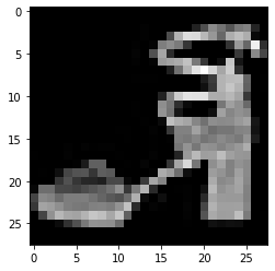
模型设计
由于任务较为简单，这里我们手搭一个CNN，而不考虑当下各种模型的复杂结构，模型构建完成后，将模型放到GPU上用于训练。

class Net(nn.Module):
    def __init__(self):
        super(Net, self).__init__()
        self.conv = nn.Sequential(
            nn.Conv2d(1, 32, 5),
            nn.ReLU(),
            nn.MaxPool2d(2, stride=2),
            nn.Dropout(0.3),
            nn.Conv2d(32, 64, 5),
            nn.ReLU(),
            nn.MaxPool2d(2, stride=2),
            nn.Dropout(0.3)
        )
        self.fc = nn.Sequential(
            nn.Linear(64*4*4, 512),
            nn.ReLU(),
            nn.Linear(512, 10)
        )
        
    def forward(self, x):
        x = self.conv(x)
        x = x.view(-1, 64*4*4)
        x = self.fc(x)
        # x = nn.functional.normalize(x)
        return x

model = Net()
model = model.cuda()
# model = nn.DataParallel(model).cuda()   # 多卡训练时的写法，之后的课程中会进一步讲解

设定损失函数
使用torch.nn模块自带的CrossEntropy损失
PyTorch会自动把整数型的label转为one-hot型，用于计算CE loss
这里需要确保label是从0开始的，同时模型不加softmax层（使用logits计算）,这也说明了PyTorch训练中各个部分不是独立的，需要通盘考虑

criterion = nn.CrossEntropyLoss()
# criterion = nn.CrossEntropyLoss(weight=[1,1,1,1,3,1,1,1,1,1])
?nn.CrossEntropyLoss # 这里方便看一下weighting等策略

设定优化器
这里我们使用Adam优化器

optimizer = optim.Adam(model.parameters(), lr=0.001)

训练和测试（验证）
各自封装成函数，方便后续调用
关注两者的主要区别：

模型状态设置
是否需要初始化优化器
是否需要将loss传回到网络
是否需要每步更新optimizer

此外，对于测试或验证过程，可以计算分类准确率

def train(epoch):
    model.train()
    train_loss = 0
    for data, label in train_loader:
        data, label = data.cuda(), label.cuda()
        optimizer.zero_grad()
        output = model(data)
        loss = criterion(output, label)
        loss.backward()
        optimizer.step()
        train_loss += loss.item()*data.size(0)
    train_loss = train_loss/len(train_loader.dataset)
    print('Epoch: {} \tTraining Loss: {:.6f}'.format(epoch, train_loss))
def val(epoch):       
    model.eval()
    val_loss = 0
    gt_labels = []
    pred_labels = []
    with torch.no_grad():
        for data, label in test_loader:
            data, label = data.cuda(), label.cuda()
            output = model(data)
            preds = torch.argmax(output, 1)
            gt_labels.append(label.cpu().data.numpy())
            pred_labels.append(preds.cpu().data.numpy())
            loss = criterion(output, label)
            val_loss += loss.item()*data.size(0)
    val_loss = val_loss/len(test_loader.dataset)
    gt_labels, pred_labels = np.concatenate(gt_labels), np.concatenate(pred_labels)
    acc = np.sum(gt_labels==pred_labels)/len(pred_labels)
    print('Epoch: {} \tValidation Loss: {:.6f}, Accuracy: {:6f}'.format(epoch, val_loss, acc))
for epoch in range(1, epochs+1):
    train(epoch)
    val(epoch)

/data1/ljq/anaconda3/envs/smp/lib/python3.8/site-packages/torch/nn/functional.py:718: UserWarning: Named tensors and all their associated APIs are an experimental feature and subject to change. Please do not use them for anything important until they are released as stable. (Triggered internally at /opt/conda/conda-bld/pytorch_1623448234945/work/c10/core/TensorImpl.h:1156.)
return torch.max_pool2d(input, kernel_size, stride, padding, dilation, ceil_mode)
Epoch: 1 Training Loss: 0.659050
Epoch: 1 Validation Loss: 0.420328, Accuracy: 0.852000
Epoch: 2 Training Loss: 0.403703
Epoch: 2 Validation Loss: 0.350373, Accuracy: 0.872300
Epoch: 3 Training Loss: 0.350197
Epoch: 3 Validation Loss: 0.293053, Accuracy: 0.893200
Epoch: 4 Training Loss: 0.322463
Epoch: 4 Validation Loss: 0.283335, Accuracy: 0.892300
Epoch: 5 Training Loss: 0.300117
Epoch: 5 Validation Loss: 0.268653, Accuracy: 0.903500
Epoch: 6 Training Loss: 0.282179
Epoch: 6 Validation Loss: 0.247219, Accuracy: 0.907200
Epoch: 7 Training Loss: 0.268283
Epoch: 7 Validation Loss: 0.242937, Accuracy: 0.907800
Epoch: 8 Training Loss: 0.257615
Epoch: 8 Validation Loss: 0.234324, Accuracy: 0.912200
Epoch: 9 Training Loss: 0.245795
Epoch: 9 Validation Loss: 0.231515, Accuracy: 0.914100
Epoch: 10 Training Loss: 0.238739
Epoch: 10 Validation Loss: 0.229616, Accuracy: 0.914400
Epoch: 11 Training Loss: 0.230499
Epoch: 11 Validation Loss: 0.228124, Accuracy: 0.915200
Epoch: 12 Training Loss: 0.221574
Epoch: 12 Validation Loss: 0.211928, Accuracy: 0.921200
Epoch: 13 Training Loss: 0.217924
Epoch: 13 Validation Loss: 0.209744, Accuracy: 0.921700
Epoch: 14 Training Loss: 0.206033
Epoch: 14 Validation Loss: 0.215477, Accuracy: 0.921400
Epoch: 15 Training Loss: 0.203349
Epoch: 15 Validation Loss: 0.215550, Accuracy: 0.919400
Epoch: 16 Training Loss: 0.196319
Epoch: 16 Validation Loss: 0.210800, Accuracy: 0.923700
Epoch: 17 Training Loss: 0.191969
Epoch: 17 Validation Loss: 0.207266, Accuracy: 0.923700
Epoch: 18 Training Loss: 0.185466
Epoch: 18 Validation Loss: 0.207138, Accuracy: 0.924200
Epoch: 19 Training Loss: 0.178241
Epoch: 19 Validation Loss: 0.204093, Accuracy: 0.924900
Epoch: 20 Training Loss: 0.176674
Epoch: 20 Validation Loss: 0.197495, Accuracy: 0.928300

模型保存
训练完成后，可以使用torch.save保存模型参数或者整个模型，也可以在训练过程中保存模型
这部分会在后面的课程中详细介绍

save_path = "./FahionModel.pkl"
torch.save(model, save_path)

十一、参考材料

[1] https://datawhalechina.github.io/thorough-pytorch/
[2] https://blog.csdn.net/weixin_42483745/article/details/125036736
[3] https://blog.csdn.net/weixin_35848967/article/details/108493217
[4] https://zhuanlan.zhihu.com/p/261134624
[5] https://zhuanlan.zhihu.com/p/34236769
[6] https://pytorch.org/docs/stable/optim.html

posted @ 2022-08-18 11:43 Xu_Lin 阅读(367) 评论(0) 编辑收藏举报

会员力量，点亮园子希望

刷新页面返回顶部

Xu_Lin

Do more; Learn more; Be more

Pytorch的主要组成模块

Pytorch的主要组成模块

一、基本配置

二、数据读入

三、模型构建

3.1 神经网络的构造

3.2 神经网络中常见的层

3.2.1 不含模型参数的层

3.2.2 含模型参数的层

3.2.3 二维卷积层

3.2.4 池化层

3.3 模型示例

3.3.1 LeNet

3.3.2 AlexNet

四、模型初始化

4.1 torch.nn.init内容

4.2 torch.nn.init使用

4.3 初始化函数的封装

五、损失函数

5.1 二分类交叉熵损失函数

5.2 交叉熵损失函数

5.3 L1损失函数

5.4 MSE损失函数

5.5 平滑L1 (Smooth L1)损失函数

5.6 目标泊松分布的负对数似然损失

5.7 KL散度

5.8 MarginRankingLoss

5.9 多标签边界损失函数

5.10 二分类损失函数

5.11 多分类的折页损失

5.12 三元组损失

5.13 HingEmbeddingLoss

5.14 余弦相似度

5.15 CTC损失函数

六、训练和评估

七、可视化

八、Pytorch优化器

8.1 Pytorch优化器

1、SGD

2、ASGD

3、AdaGrad

4、AdaDelta

5、Rprop

6、RMSProp

7、Adam(AMSGrad)

8、Adamax

9、Nadam

10、SparseAdam

11、AdamW

12、L-BFGS

13、Radam

8.2 实际操作

8.3 输出结果

8.4 实验

九、Pytorch学习率衰减

学习率衰减

如何调整学习率

按照自定义函数进行学习率衰减

按照自定义因子进行学习率衰减

间隔N个epoch之后进行衰减

训练指定的epoch之后进行衰减

指数衰减

余弦退火衰减

带热重启的余弦退火衰减

在训练进入平台期后进行学习率衰减

OneCycleLR

CyclicLR

十、完整示例

十一、参考材料

公告