TensorFlow作业

TensorFlowd学习报告：

Tensor（张量）意味着N维数组，Flow（流）意味着基于数据流图的计算.数据流图中的图就是我们所说的有向图,我们知道,在图这种数据结构中包含两种基本元素:节点和边.这两种元素在数据流图中有自己各自的作用。节点用来表示要进行的数学操作,另外,任何一种操作都有输入/输出,因此它也可以表示数据的输入的起点/输出的终点。边表示节点与节点之间的输入/输出关系,一种特殊类型的数据沿着这些边传递.这种特殊类型的数据在TensorFlow被称之为tensor,即张量,所谓的张量通俗点说就是多维数组.当我们向这种图中输入张量后,节点所代表的操作就会被分配到计算设备完成计算。此外，TensorFlowd还分别具有一以下四个特性：灵活性、可移植性、多语言支持和高效性。

实验：

# TensorFlow and tf.keras
import tensorflow as tf
from tensorflow import keras

# Helper libraries
import numpy as np
import matplotlib.pyplot as plt

print(tf.__version__)

fashion_mnist = keras.datasets.fashion_mnist

(train_images, train_labels), (test_images, test_labels) = fashion_mnist.load_data()

class_names = ['T-shirt/top', 'Trouser', 'Pullover', 'Dress', 'Coat',
'Sandal', 'Shirt', 'Sneaker', 'Bag', 'Ankle boot']

train_images.shape
len(train_labels)
train_labels
test_images.shape
len(test_labels)

plt.figure()
plt.imshow(train_images[0])
plt.colorbar()
plt.grid(False)
plt.show()

train_images = train_images / 255.0

test_images = test_images / 255.0

plt.figure(figsize=(10,10))
for i in range(25):
plt.subplot(5,5,i+1)
plt.xticks([])
plt.yticks([])
plt.grid(False)
plt.imshow(train_images[i], cmap=plt.cm.binary)
plt.xlabel(class_names[train_labels[i]])
plt.show()

model = keras.Sequential([
keras.layers.Flatten(input_shape=(28, 28)),
keras.layers.Dense(128, activation='relu'),
keras.layers.Dense(10)
])

model.compile(optimizer='adam',
loss=tf.keras.losses.SparseCategoricalCrossentropy(from_logits=True),
metrics=['accuracy'])

model.fit(train_images, train_labels, epochs=10)

test_loss, test_acc = model.evaluate(test_images, test_labels, verbose=2)

print('\nTest accuracy:', test_acc)

probability_model = tf.keras.Sequential([model,
tf.keras.layers.Softmax()])
predictions = probability_model.predict(test_images)
predictions[0]
np.argmax(predictions[0])
test_labels[0]

def plot_image(i, predictions_array, true_label, img):
predictions_array, true_label, img = predictions_array, true_label[i], img[i]
plt.grid(False)
plt.xticks([])
plt.yticks([])

plt.imshow(img, cmap=plt.cm.binary)

predicted_label = np.argmax(predictions_array)
if predicted_label == true_label:
color = 'blue'
else:
color = 'red'

plt.xlabel("{} {:2.0f}% ({})".format(class_names[predicted_label],
100*np.max(predictions_array),
class_names[true_label]),
color=color)

def plot_value_array(i, predictions_array, true_label):
predictions_array, true_label = predictions_array, true_label[i]
plt.grid(False)
plt.xticks(range(10))
plt.yticks([])
thisplot = plt.bar(range(10), predictions_array, color="#777777")
plt.ylim([0, 1])
predicted_label = np.argmax(predictions_array)

thisplot[predicted_label].set_color('red')
thisplot[true_label].set_color('blue')

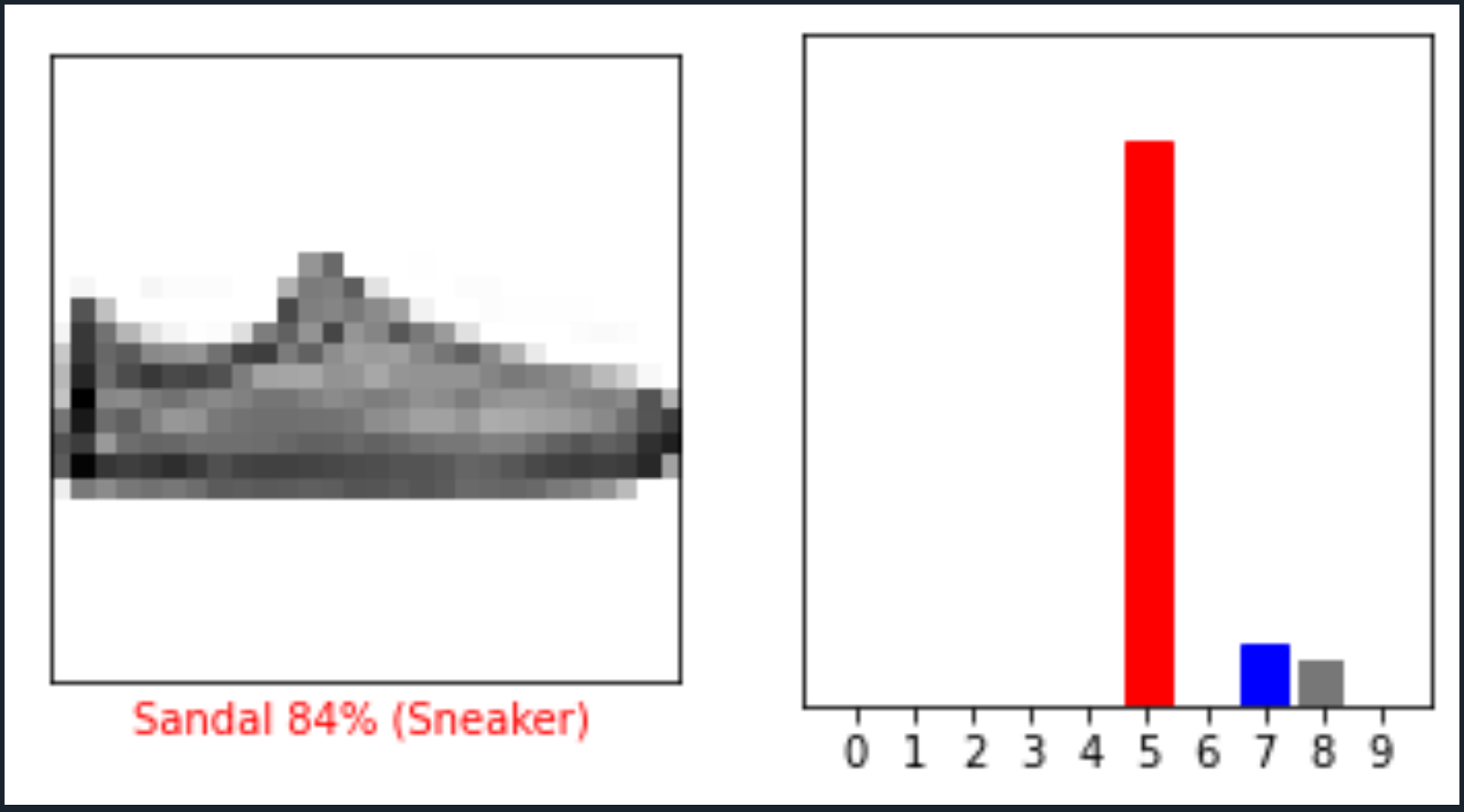
i = 0
plt.figure(figsize=(6,3))
plt.subplot(1,2,1)
plot_image(i, predictions[i], test_labels, test_images)
plt.subplot(1,2,2)
plot_value_array(i, predictions[i], test_labels)
plt.show()

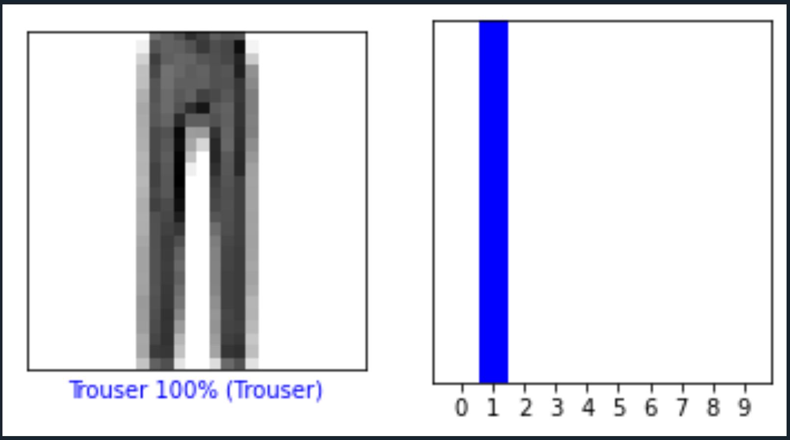
i = 12
plt.figure(figsize=(6,3))
plt.subplot(1,2,1)
plot_image(i, predictions[i], test_labels, test_images)
plt.subplot(1,2,2)
plot_value_array(i, predictions[i], test_labels)
plt.show()

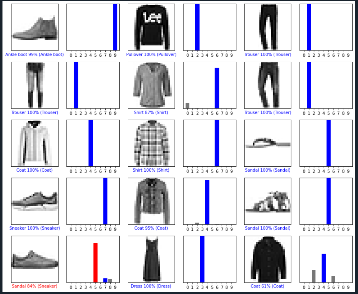
num_rows = 5
num_cols = 3
num_images = num_rows*num_cols
plt.figure(figsize=(2*2*num_cols, 2*num_rows))
for i in range(num_images):
plt.subplot(num_rows, 2*num_cols, 2*i+1)
plot_image(i, predictions[i], test_labels, test_images)
plt.subplot(num_rows, 2*num_cols, 2*i+2)
plot_value_array(i, predictions[i], test_labels)
plt.tight_layout()
plt.show()

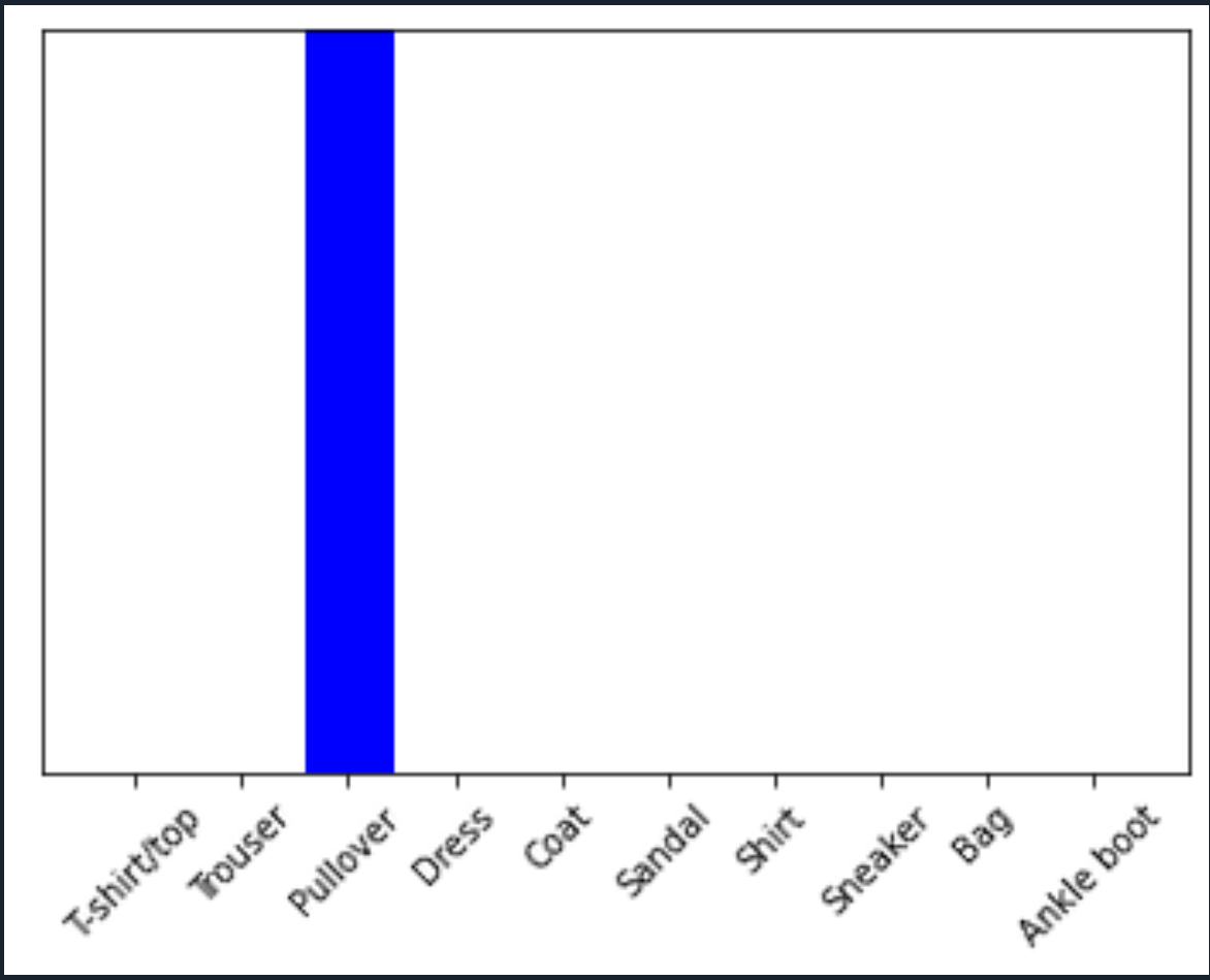
img = test_images[1]

print(img.shape)

img = (np.expand_dims(img,0))

print(img.shape)

predictions_single = probability_model.predict(img)

print(predictions_single)

plot_value_array(1, predictions_single[0], test_labels)
_ = plt.xticks(range(10), class_names, rotation=45)

np.argmax(predictions_single[0])

结果：

 

课后作业：

1，卷积中的局部连接：层间神经只有局部范围内的连接，在这个范围内采用全连接的方式，超过这个范围的神经元则没有连接；连接与连接之间独立参数，相比于去全连接减少了感受域外的连接，有效减少参数规模。全连接：层间神经元完全连接，每个输出神经元可以获取到所有神经元的信息，有利于信息汇总，常置于网络末尾；连接与连接之间独立参数，大量的连接大大增加模型的参数规模。

2，利用快速傅里叶变换把图片和卷积核变换到频域，频域把两者相乘，把结果利用傅里叶逆变换得到特征图。

3，池化操作的作用：对输入的特征图进行压缩,一方面使特征图变小,简化网络计算复杂度;一方面进行特征压缩,提取主要特征。激活函数的作用：用来加入非线性因素的，解决线性模型所不能解决的问题。

4，消除数据之间的量纲差异，便于数据利用与快速计算。

5，寻找损失函数的最低点，就像我们在山谷里行走，希望找到山谷里最低的地方。那么如何寻找损失函数的最低点呢？在这里，我们使用了微积分里导数，通过求出函数导数的值，从而找到函数下降的方向或者是最低点（极值点）。损失函数里一般有两种参数，一种是控制输入信号量的权重(Weight, 简称  ），另一种是调整函数与真实值距离的偏差（Bias，简称  ）。我们所要做的工作，就是通过梯度下降方法，不断地调整权重  和偏差b，使得损失函数的值变得越来越小。而随机梯度下降算法只随机抽取一个样本进行梯度计算。