Computability and Complexity

Computability and Complexity https://plato.stanford.edu/entries/computability/

First published Thu Jun 24, 2004; substantive revision Wed Sep 2, 2015

A mathematical problem is computable if it can be solved in principle by a computing device. Some common synonyms for “computable” are “solvable”, “decidable”, and “recursive”. Hilbert believed that all mathematical problems were solvable, but in the 1930’s Gödel, Turing, and Church showed that this is not the case. There is an extensive study and classification of which mathematical problems are computable and which are not. In addition, there is an extensive classification of computable problems into computational complexity classes according to how much computation—as a function of the size of the problem instance—is needed to answer that instance. It is striking how clearly, elegantly, and precisely these classifications have been drawn.

1. What can be computed in principle? Introduction and History

In the 1930’s, well before there were computers, various mathematicians from around the world invented precise, independent definitions of what it means to be computable. Alonzo Church defined the Lambda calculus, Kurt Gödel defined Recursive functions, Stephen Kleene defined Formal systems, Markov defined what became known as Markov algorithms, Emil Post and Alan Turing defined abstract machines now known as Post machines and Turing machines.

Surprisingly, all of these models are exactly equivalent: anything computable in the lambda calculus is computable by a Turing machine and similarly for any other pairs of the above computational systems. After this was proved, Church expressed the belief that the intuitive notion of “computable in principle” is identical to the above precise notions. This belief, now called the “Church-Turing Thesis”, is uniformly accepted by mathematicians.

Part of the impetus for the drive to codify what is computable came from the mathematician David Hilbert. Hilbert believed that all of mathematics could be precisely axiomatized. He felt that once this was done, there would be an “effective procedure”, i.e., an algorithm that would take as input any precise mathematical statement, and, after a finite number of steps, decide whether the statement was true or false. Hilbert was asking for what would now be called a decision procedure for all of mathematics.

As a special case of this decision problem, Hilbert considered the validity problem for first-order logic. First-order logic is a mathematical language in which most mathematical statements can be formulated. Every statement in first-order logic has a precise meaning in every appropriate logical structure, i.e., it is true or false in each such structure. Those statements that are true in every appropriate structure are called valid. Those statements that are true in some structure are called satisfiable. Notice that a formula, $φ$

Hilbert called the validity problem for first-order logic, the entscheidungsproblem. In a textbook, Principles of Mathematical Logic by Hilbert and Ackermann, the authors wrote, “The Entscheidungsproblem is solved when we know a procedure that allows for any given logical expression to decide by finitely many operations its validity or satisfiability.… The entscheidungsproblem must be considered the main problem of mathematical logic.” (Böerger, Grädel, & Gurevich 1997).

In his 1930 Ph.D. thesis, Gödel presented a complete axiomatization of first-order logic, based on the Principia Mathematica by Whitehead and Russell (Gödel 1930). Gödel proved his Completeness Theorem, namely that a formula is provable from the axioms if and only if it is valid. Gödel’s Completeness theorem was a step towards the resolution of Hilbert’s entscheidungsproblem.

In particular, since the axioms are easily recognizable, and rules of inference very simple, there is a mechanical procedure that can list out all proofs. Note that each line in a proof is either an axiom, or follows from previous lines by one of the simple rules. For any given string of characters, we can tell if it is a proof. Thus we can systematically list all strings of characters of length 1, 2, 3, and so on, and check whether each of these is a proof. If so, then we can add the proof’s last line to our list of theorems. In this way, we can list out all theorems, i.e., exactly all the valid formulas of first-order logic, can be listed out by a simple mechanical procedure. More precisely, the set of valid formulas is the range of a computable function. In modern terminology we say that the set of valid formulas of first-order logic is recursively enumerable (r.e.).

Gödel’s Completeness theorem was not sufficient, however, to give a positive solution to the entscheidungsproblem. Given a formula, $φ$

A year later, in 1931, Gödel shocked the mathematical world by proving his Incompleteness Theorem: there is no complete and computable axiomatization of the first-order theory of the natural numbers. That is, there is no reasonable list of axioms from which we can prove exactly all true statements of number theory (Gödel 1931).

A few years later, Church and Turing independently proved that the entscheidungsproblem is unsolvable. Church did this by using the methods of Gödel’s Incompleteness Theorem to show that the set of satisfiable formulas of first-order logic is not r.e., i.e., they cannot be systematically listed out by a function computable by the lambda calculus. Turing introduced his machines and proved many interesting theorems some of which we will discuss in the next section. In particular, he proved the unsolvability of the halting problem. He obtained the unsolvability of the entscheidungsproblem as a corollary.

Hilbert was very disappointed because his program towards a decision procedure for all of mathematics was proved impossible. However, as we will see in more detail in the rest of this article, a vast amount was learned about the fundamental nature of computation.

2. Turing Machines

In his 1936 paper, “On Computable Numbers, with an Application to the Entscheidungsproblem”, Alan Turing introduced his machines and established their basic properties.

He thought clearly and abstractly about what it would mean for a machine to perform a computational task. Turing defined his machines to consist of the following:

a finite set, $Q$
a potentially infinite tape, consisting of consecutive cells, $σ_{1}, σ_{2}, σ_{3}$
a read/write tape head, $h \geq 1$
a transition function, $δ : Q \times Σ \to Q \times Σ \times {- 1, 0, 1}$

The linear nature of its memory tape, as opposed to random access memory, is a limitation on computation speed but not power: a Turing machine can find any memory location, i.e., tape cell, but this may be time consuming because it has to move its head step by step along its tape.

The beauty of Turing machines is that the model is extremely simple, yet nonetheless, extremely powerful. A Turing machine has potentially infinite work space so that it can process arbitrarily large inputs, e.g., multiply two huge numbers, but it can only read or write a bounded amount of information, i.e., one symbol, per step. Even before Turing machines and all the other mathematical models of computation were proved equivalent, and before any statement of the Church-Turing thesis, Turing argued convincingly that his machines were as powerful as any possible computing device.

2.1 Universal Machines

Each Turing machine can be uniquely described by its transition table: for each state, $q$

Turing showed that he could build a Turing machine, $U$

U (i, w) = M i (w)

Turing’s construction of a universal machine gives the most fundamental insight into computation: one machine can run any program whatsoever. No matter what computational tasks we may need to perform in the future, a single machine can perform them all. This is the insight that makes it feasible to build and sell computers. One computer can run any program. We don’t need to buy a new computer every time we have a new problem to solve. Of course, in the age of personal computers, this fact is such a basic assumption that it may be difficult to step back and appreciate it.

2.2 The Halting Problem

Because they were designed to embody all possible computations, Turing machines have an inescapable flaw: some Turing machines on certain inputs never halt. Some Turing machines do not halt for silly reasons, for example, we can mis-program a Turing machine so that it gets into a tight loop, for example, in state 17 looking at a 1 it might go to state 17, write a 1 and displace its head by 0. Slightly less silly, we can reach a blank symbol, having only blank symbols to the right, and yet keep staying in the same state, moving one step to the right, and looking for a “1”. Both of those cases of non-halting could be easily detected and repaired by a decent compiler. However, consider the Turing machine $M_{F}$

2.3 Computable Functions and Enumerability

Since a Turing machine might not halt on certain inputs, we have to be careful in how we define functions computable by Turing machines. Let the natural numbers, $N$

Let $M$

If we start the Turing machine $M$

Now we can formally define what it means for a set to be recursively enumerable (r.e.) which we earlier described informally. Let $S \subseteq N$

S = {M (n) ∣ n \in N; M (n) \neq↗} .

Thus, $S$

Let the notation $P (n) ↓$

L (P) = {n ∣ P (n) ↓} .

The above argument shows that if a set $S$

We say that a set, $S$

For $S \subseteq N$

2.4 The Unsolvability of the Halting Problem

Turing asked whether every set of natural numbers is decidable. It is easy to see that the answer is, “no”, by the following counting argument. There are uncountably many subsets of $N$

Turing actually constructed a non-decidable set. As we will see, he did this using a diagonal argument. The diagonal argument goes back to Georg Cantor who used it to show that the real numbers are uncountable. Gödel used a similar diagonal argument in his proof of the Incompleteness Theorem in which he constructed a sentence, $J$

Turing constructed a diagonal halting set, $K$

K = {n ∣ M n (n) ↓} .

That is, $K$

It is not hard to see that $K$

n \notin K \Leftrightarrow M d (n) ↓

But consider what happens when we substitute $d$

d \notin K \Leftrightarrow M d (d) ↓ .

However, the definition of $K$

d \in K \Leftrightarrow M d (d) ↓ .

Thus we have that

d \in K \Leftrightarrow d \notin K,

which is a contradiction. Thus our assumption that $K$

3. Primitive Recursive Functions

We next define the class of Primitive Recursive Functions. This is a very interesting class of functions described in paper by Skolem (1923) and used by Gödel in his proof of the Incompleteness Theorem. We are interested in functions $f$

We begin with the three initial primitive recursive functions:

$ζ$
$η$
$σ$

Now consider the following two operations:

Composition: if $f$ $h (x 1, \dots, x k) = f (g 1 (w 1), \dots, g a (w a))$
where each $w_{i}$
Primitive recursion: if $f$ $h (0, x 1, \dots, x k) h (n + 1, x 1, \dots, x k) =$

Here composition is the natural way to combine functions, and primitive recursion is a restricted kind of recursion in which $h$

Define the primitive recursive functions to be the smallest class of functions that contains the Initial functions and is closed under Composition and Primitive Recursion. The set of primitive recursive functions is equal to the set of functions computed using bounded iteration (Meyer & Ritchie 1967), i.e. the set of functions definable in the language Bloop from (Hofstadter 1979).

The primitive recursive functions have a very simple definition and yet they are extremely powerful. Gödel proved inductively that every primitive recursive function can be simply represented in first-order number theory. He then used the primitive recursive functions to encode formulas and even sequences of formulas by numbers. He finally used the primitive recursive functions to compute properties of the represented formulas including that a formula was well formed, a sequence of formulas was a proof, and that a formula was a theorem.

It takes a long series of lemmas to show how powerful the primitive recursive functions are. The following are a few examples showing that addition, multiplication, and exponentiation are primitive recursive.

Define the addition function, $P (x, y)$

P (0, y) P (n + 1, y) = η (y) = σ (P (n, y))

(Note that this fits into the definition of primitive recursion because the function $g (x_{1}, x_{2}, x_{3}) = η (σ (x_{1}))$

Next, define the multiplication function, $T (x, y)$

T (0, y) T (n + 1, y) = ζ () = P (T (n, y), y) .

Next, we define the exponential function, $E (x, y)$

R (0, y) R (n + 1, y) = σ (ζ ()) = T (R (n, y), y) .

Finally we can define $E (x, y) = R (η (y), η (x))$

The exponential function, $E$

H (0, y) H (n + 1, y) = y = E (2, H (n, y))

Thus $H (2, 2) = 2^{4} = 16, H (3, 3) = 2^{256}$

3.1 Recursive Functions

The set of primitive recursive functions is a huge class of computable functions. In fact, they can be characterized as the set of functions computable in time that is some primitive recursive function of $n$

However, the primitive recursive functions do not include all functions computable in principle. To see this, we can again use diagonalization. We can systematically encode all definitions of primitive recursive functions of arity 1, calling them $p_{1}, p_{2}, p_{3}$

We can then build a Turing machine to compute the value of the following diagonal function, $D (n) = p_{n} (n) + 1$

Notice that $D$

p d (d) = p d (d) + 1,

which is a contradiction. Therefore, $D$

Alas, the above diagonal argument works on any class of total functions that could be considered a candidate for the class of all computable functions. The only way around this, if we want all functions computable in principle, not just in practice, is to add some kind of unbounded search operation. This is what Gödel did to extend the primitive recursive functions to the recursive functions.

Define the unbounded minimization operator, $μ$

For $i = 0$

if $f (i, x_{1}, \dots, x_{k}) = 1$

$}$

Thus if $f (i, x_{1}, \dots, x_{k}) = 1$

Gödel defined the set of Recursive functions to be the closure of the initial primitive recursive functions under composition, primitive recursion, and $μ$

4. Computational Complexity: Functions Computable in Practice

During World War II, Turing helped design and build a specialized computing device called the Bombe at Bletchley Park. He used the Bombe to crack the German “Enigma” code, greatly aiding the Allied cause [Hodges, 1992]. By the 1960’s computers were widely available in industry and at universities. As algorithms were developed to solve myriad problems, some mathematicians and scientists began to classify algorithms according to their efficiency and to search for best algorithms for certain problems. This was the beginning of the modern theory of computation.

In this section we are dealing with complexity instead of computability, and all the Turing machines that we consider will halt on all their inputs. Rather than accepting by halting, we will assume that a Turing machine accepts by outputting “1” and rejects by outputting “0”, thus we redefine the set accepted by a total machine, $M$

L (M) = {n ∣ M (n) = 1} .

The time that an algorithm takes depends on the input and the machine on which it is run. The first important insight in complexity theory is that a good measure of the complexity of an algorithm is its asymptotic worst-case complexity as a function of the size of the input, $n$

For an input, $w$

For any function $T : N \to N$

T I M E [T (n)] = {A ∣ A = L (M) for some M that runs in time T (n)} .

Alan Cobham and Jack Edmonds identified the complexity class, $P$

P = ⋃ i = 1, 2, \dots T I M E [n i]

Any problem not in $P$

Many important complexity classes besides P have been defined and studied; a few of these are $N P$

Perhaps the most interesting of the above classes is NP: nondeterministic polynomial time. The definition comes not from a real machine, but rather a mathematical abstraction. A nondeterministic Turing machine, $N$

NP is sometimes described as the set of problems, $S$

There has been a large study of algorithms and the complexity of many important problems is well understood. In particular reductions between problems have been defined and used to compare the relative difficulty of two problems. Intuitively, we say that $A$

Remarkably, a high percentage of naturally occurring computational problems turn out to be complete for one of the above classes. (A problem, $A$

The reason for this completeness phenomenon has not been adequately explained. One plausible explanation is that natural computational problems tend to be universal in the sense of Turing’s universal machine. A universal problem in a certain complexity class can simulate any other problem in that class. The reason that the class NP is so well studied is that a large number of important practical problems are NP complete, including Subset Sum. None of these problems is known to have an algorithm that is faster than exponential time, although some NP-complete problems admit feasible approximations to their solutions.

A great deal remains open about computational complexity. We know that strictly more of a particular computational resource lets us solve strictly harder problems, e.g. $T I M E [n]$

P \subseteq N P \subseteq P S P A C E \subseteq E X P T I M E

However, while it seems clear that $P$

There is an extensive theory of computational complexity. This entry briefly describes the area, putting it into the context of the question of what is computable in principle versus in practice. For readers interested in learning more about complexity, there are excellent books, for example, [Papadimitriou, 1994] and [Arora and Barak, 2009]. There is also the entry on Computational Complexity Theory.

4.1 Significance of Complexity

The following diagram maps out all the complexity classes we have discussed and a few more as well. The diagram comes from work in Descriptive Complexity [Immerman, 1999] which shows that all important complexity classes have descriptive characterizations. Fagin began this field by proving that NP = SO $\exists$

Vardi and the author of this entry later independently proved that P = FO(LFP): a property is in P iff it is expressible in first-order logic plus a least fixed-point operator (LFP) which formalizes the power to define new relations by induction. A captivating corollary of this is that P = NP iff SO = FO(LFP). That is, P is equal to NP iff every property expressible in second order logic is already expressible in first-order logic plus inductive definitions. (The languages in question are over finite ordered input structures. See [Immerman, 1999] for details.)

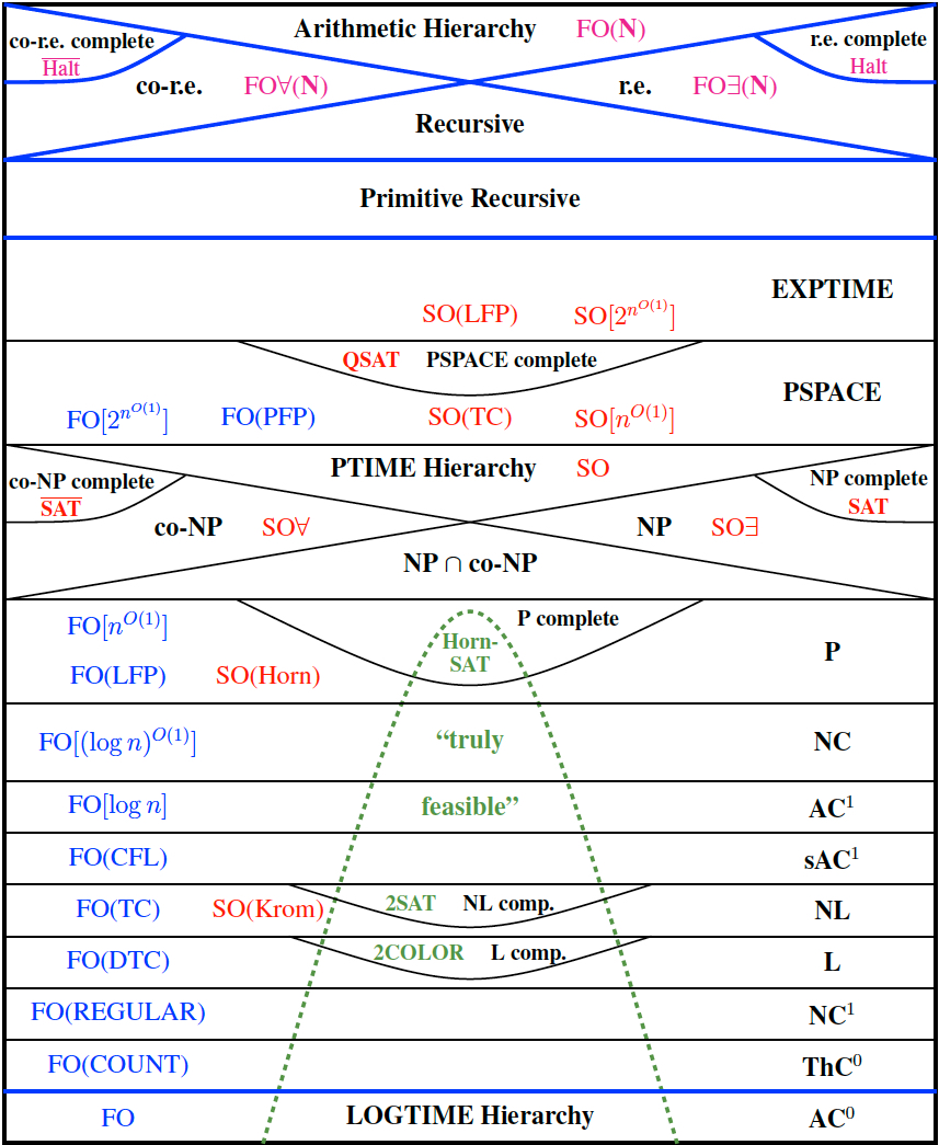
The World of Computability and Complexity

The top right of the diagram shows the recursively enumerable (r.e.) problems; this includes r.e.-complete problems such as the halting problem (Halt). On the left is the set of co-r.e. problems including the co-r.e.-complete problem $\bar{H a l t}$

Moving toward the bottom of the diagram, there is a region marked with a green dotted line labelled “truly feasible”. Note that this is not a mathematically defined class, but rather an intuitive notion of those problems that can be solved exactly, for all the instances of reasonable size, within a reasonable amount of time, using a computer that we can afford. (Interestingly, as the speed of computers has dramatically increased over the years, our expectation of how large an instance we should be able to handle has increased accordingly. Thus, the boundary of what is “truly feasible” changes more slowly than the increase of computer speed might suggest.)

As mentioned before, P is a good mathematical wrapper for the set of feasible problems. There are problems in P requiring $n^{1, 000}$

In practice the asympototic complexity of naturally occurring problems tends to be the key issue determining whether or not they are feasible. A problem with complexity $17 n$

Remarkably, natural problems tend to be complete for important complexity classes, namely the ones in the diagram and only a very few others. This fascinating phenomenon means that algorithms and complexity are more than abstract concepts; they are important at a practical level. We have had remarkable success in proving that our problem of interest is complete for a well-known complexity class. If the class is contained in P, then we can usually just look up a known efficient algorithm. Otherwise, we must look at simplifications or approximations of our problem which may be feasible.

There is a rich theory of the approximability of NP optimization problems (See [Arora & Barak, 2009]). For example, the Subset Sum problem mentioned above is an NP-complete problem. Most likely it requires exponential time to tell whether a given Subset Sum problem has an exact solution. However, if we only want to see if we can reach the target up to a fixed number of digits of accuracy, then the problem is quite easy, i.e., Subset Sum is hard, but very easy to approximate.

Even the r.e.-complete Halting problem has many important feasible subproblems. Given a program, it is in general not possible to figure out what it does and whether or not it eventually halts. However, most programs written by programmers or students can be automatically analyzed, optimized and even corrected by modern compilers and model checkers.

The class NP is very important practically and philosophically. It is the class of problems, $S$

The boolean satisfiability problem, SAT, was the first problem proved NP complete [Cook, 1971], i.e., it is a hardest NP problem. The fact that SAT is NP complete means that all problems in NP are reducible to SAT. Over the years, researchers have built very efficient SAT solvers which can quickly solve many SAT instances – i.e., find a satisfying assignment or prove that there is none -- even for instances with millions of variables. Thus, SAT solvers are being used as general purpose problem solvers. On the other hand, there are known classes of small instances for which current SAT solvers fail. Thus part of the P versus NP question concerns the practical and theoretical complexity of SAT [Nordström, 2015].

Bibliography

Arora, Sanjeev and Boaz Barak, 2009, Computational Complexity: A Modern Approach, New York: Cambridge University Press.
Church, Alonzo, 1933, “A Set of Postulates for the Foundation of Logic (Second Paper)”, Annals of Mathematics (Second Series), 33: 839–864.
–––, 1936, “An Unsolvable Problem of Elementary Number Theory,” American Journal of Mathematics, 58: 345–363..
–––, 1936, “A Note on the Entscheidungsproblem,” Journal of Symbolic Logic, 1: 40–41; correction 1, 101–102.
Böerger, Egon, Erich Grädel, and Yuri Gurevich, 1997, The Classical Decision Problem, Heidelberg: Springer.
Cobham, Alan, 1964, “The Intrinsic Computational Difficulty of Functions,” Proceedings of the 1964 Congress for Logic, Mathematics, and Philosophy of Science, Amsterdam: North-Holland 24–30.
Cook, Stephen, 1971, “The Complexity of Theorem Proving Procedures,” Proceedings of the Third Annual ACM STOC Symposium, Shaker Heights, Ohio, 151–158.
Davis, Martin, 2000,The Universal Computer: the Road from Leibniz to Turing, New York: W. W. Norton & Company.
Edmonds, Jack, 1965, “Paths, Trees and Flowers,” Canadian Journal of Mathematics, 17: 449–467.
Enderton, Herbert B., 1972, A Mathematical Introduction to Logic, New York: Academic Press.
Fagin, Ronald, 1974, “Generalized First-Order Spectra and Polynomial-Time Recognizable Sets,” in Complexity of Computation, R. Karp(ed.), SIAM-AMS Proc, 7: 27–41.
Garey, Michael and David S. Johnson, 1979, Computers and Intractability, New York: Freeman.
Gödel, Kurt, 1930, “The Completeness of the Axioms of the Functional Calculus,” in van Heijenoort 1967, 582–591.
–––, 1931, “On Formally Undecidable Propositions of Principia Mathematica and Related Systems I,” in van Heijenoort, 1967, 592–617.
Hartmanis, Juris, 1989, “Overview of computational Complexity Theory” in J. Hartmanis (ed.), Computational Complexity Theory, Providence: American Mathematical Society, 1–17.
Hilbert and Ackermann, 1928/1938, Grundzüge der theoretischen Logik, Springer. English translation of the 2nd edition: Principles of Mathematical Logic, New York: Chelsea Publishing Company, 1950.
Hodges, Andrew, 1992, Alan Turing: the Enigma, London: Random House.
Hofstadter, Douglas, 1979, Gödel, Escher, Bach: an Eternal Golden Braid, New York: Basic Books.
Hopcroft, John E., 1984, “Turing Machines”, Scientific American, 250(5): 70–80.
Immerman, Neil, 1999, Descriptive Complexity, New York: Springer.
Karp, Richard, 1972, “Reducibility Among Combinatorial Problems,”, in Complexity of Computations, R.E. Miller and J.W. Thatcher (eds.), New York: Plenum Press, 85–104.
Kleene, Stephen C., 1935, “A Theory of Positive Integers in Formal Logic,” American Journal of Mathematics, 57: 153–173, 219–244.
–––, 1950, Introduction to Metamathematics, Princeton: Van Nostrand.
Levin, Leonid, 1973, “Universal search problems,” Problemy Peredachi Informatsii, 9(3): 265–266; partial English translation in B.A.Trakhtenbrot, 1984, “A Survey of Russian Approaches to Perebor (Brute-force Search) Algorithms,” IEEE Annals of the History of Computing, 6(4): 384–400.
Markov, A.A., 1960, “The Theory of Algorithms,” American Mathematical Society Translations (Series 2), 15: 1–14.
Meyer, Albert and Dennis Ritchie, 1967, “The Complexity of Loop Programs,” Proceedings of the 22nd National ACM Conference, Washington, D.C., 465–470.
Nordström, Jakob, 2015, “On the Interplay Between Proof Complexity and SAT Solving,” SIGLOG News, 2(3):18–44.
Papadimitriou, Christos H., 1994, Computational Complexity, Reading, MA: Addison-Wesley.
Péter, Rózsa. 1967, Recursive Functions, translated by István Földes, New York: Academic Press.
Post, Emil, 1936, “Finite Combinatory Processes – Formulation I,” Journal of Symbolic Logic, 1: 103–105.
Rogers, Hartley Jr., 1967, Theory of Recursive Functions and Effective Computability, New York: McGraw-Hill.
Skolem, Thoralf, 1923, “The foundations of elementary arithmetic established by means of the recursive mode of thought,” in van Heijenoort (1967): 302–33.
Turing, A. M., 1936–7, “On Computable Numbers, with an Application to the Entscheidungsproblem”, Proceedings of the London Mathematical Society, 2(42): 230–265 [Preprint available online].
van Heijenoort, Jean , ed., 1967, From Frege To Gödel: A Source Book in Mathematical Logic, 1879–1931, Cambridge, MA: Harvard University Press.
Whitehead, Alfred North and Bertrand Russell, 1910–1913, Principia Mathematica, first edition, Cambridge: Cambridge University Press.

Academic Tools

How to cite this entry.

Preview the PDF version of this entry at the Friends of the SEP Society.

Look up this entry topic at the Internet Philosophy Ontology Project (InPhO).

Enhanced bibliography for this entry at PhilPapers, with links to its database.

Other Internet Resources

Descriptive Complexity: a webpage describing research in Descriptive Complexity which is Computational Complexity from a Logical Point of View (with a diagram showing the World of Computability and Complexity). Maintained by Neil Immerman, University of Massachusetts, Amherst.
Mass, Size, and Density of the Universe, from the National Solar Observatory/Sacramento Peak.

posted @ 2020-11-01 12:00 hjlweilong 阅读(189) 评论(0) 编辑收藏举报

会员力量，点亮园子希望

刷新页面返回顶部

	How to cite this entry.
	Preview the PDF version of this entry at the Friends of the SEP Society.
	Look up this entry topic at the Internet Philosophy Ontology Project (InPhO).
	Enhanced bibliography for this entry at PhilPapers, with links to its database.