Pandas快速入门

This is a short introduction to pandas, geared mainly for new users. You can see more complex recipes in the Cookbook

Customarily, we import as follows:

In [1]: import pandas as pd

In [2]: import numpy as np

In [3]: import matplotlib.pyplot as plt

Object Creation

See the Data Structure Intro section

------------------------------------------------------------------------------------------------------------

Intro to Data Structures

We’ll start with a quick, non-comprehensive overview of the fundamental data structures in pandas to get you started. The fundamental behavior about data types, indexing, and axis labeling / alignment apply across all of the objects. To get started, import numpy and load pandas into your namespace:

In [1]: import numpy as np

In [2]: import pandas as pd

Here is a basic tenet to keep in mind: data alignment is intrinsic. The link between labels and data will not be broken unless done so explicitly by you.

We’ll give a brief intro to the data structures, then consider all of the broad categories of functionality and methods in separate sections.

Series

Series is a one-dimensional labeled array capable of holding any data type (integers, strings, floating point numbers, Python objects, etc.). The axis labels are collectively referred to as the index. The basic method to create a Series is to call:

>>> s = pd.Series(data, index=index)

Here, data can be many different things:

• a Python dict
• an ndarray
• a scalar value (like 5)

The passed index is a list of axis labels. Thus, this separates into a few cases depending on what data is:

From ndarray

If data is an ndarray, index must be the same length as data. If no index is passed, one will be created having values [0, ..., len(data) - 1].

In [3]: s = pd.Series(np.random.randn(5), index=['a', 'b', 'c', 'd', 'e'])

In [4]: s
Out[4]: 
a    0.4691
b   -0.2829
c   -1.5091
d   -1.1356
e    1.2121
dtype: float64

In [5]: s.index
Out[5]: Index(['a', 'b', 'c', 'd', 'e'], dtype='object')

In [6]: pd.Series(np.random.randn(5))
Out[6]: 
0   -0.1732
1    0.1192
2   -1.0442
3   -0.8618
4   -2.1046
dtype: float64

Note

 

pandas supports non-unique index values. If an operation that does not support duplicate index values is attempted, an exception will be raised at that time. The reason for being lazy is nearly all performance-based (there are many instances in computations, like parts of GroupBy, where the index is not used).

From dict

If data is a dict, if index is passed the values in data corresponding to the labels in the index will be pulled out. Otherwise, an index will be constructed from the sorted keys of the dict, if possible.

In [7]: d = {'a' : 0., 'b' : 1., 'c' : 2.}

In [8]: pd.Series(d)
Out[8]: 
a    0.0
b    1.0
c    2.0
dtype: float64

In [9]: pd.Series(d, index=['b', 'c', 'd', 'a'])
Out[9]: 
b    1.0
c    2.0
d    NaN
a    0.0
dtype: float64

Note

 

NaN (not a number) is the standard missing data marker used in pandas

From scalar value If data is a scalar value, an index must be provided. The value will be repeated to match the length of index

In [10]: pd.Series(5., index=['a', 'b', 'c', 'd', 'e'])
Out[10]: 
a    5.0
b    5.0
c    5.0
d    5.0
e    5.0
dtype: float64

Series is ndarray-like

Series acts very similarly to a ndarray, and is a valid argument to most NumPy functions. However, things like slicing also slice the index.

In [11]: s[0]
Out[11]: 0.46911229990718628

In [12]: s[:3]
Out[12]: 
a    0.4691
b   -0.2829
c   -1.5091
dtype: float64

In [13]: s[s > s.median()]   #先排序，后中值
Out[13]: 
a    0.4691
e    1.2121
dtype: float64

In [14]: s[[4, 3, 1]]
Out[14]: 
e    1.2121
d   -1.1356
b   -0.2829
dtype: float64

In [15]: np.exp(s)
Out[15]: 
a    1.5986
b    0.7536
c    0.2211
d    0.3212
e    3.3606
dtype: float64

We will address array-based indexing in a separate section.

Series is dict-like

A Series is like a fixed-size dict in that you can get and set values by index label:

In [16]: s['a']
Out[16]: 0.46911229990718628

In [17]: s['e'] = 12.

In [18]: s
Out[18]: 
a     0.4691
b    -0.2829
c    -1.5091
d    -1.1356
e    12.0000
dtype: float64

In [19]: 'e' in s
Out[19]: True

In [20]: 'f' in s
Out[20]: False

If a label is not contained, an exception is raised:

>>> s['f']
KeyError: 'f'

Using the get method, a missing label will return None or specified default:

In [21]: s.get('f')

In [22]: s.get('f', np.nan)
Out[22]: nan

See also the section on attribute access.

Vectorized operations and label alignment with Series

When doing data analysis, as with raw NumPy arrays looping through Series value-by-value is usually not necessary. Series can also be passed into most NumPy methods expecting an ndarray.

In [23]: s + s
Out[23]: 
a     0.9382
b    -0.5657
c    -3.0181
d    -2.2713
e    24.0000
dtype: float64

In [24]: s * 2
Out[24]: 
a     0.9382
b    -0.5657
c    -3.0181
d    -2.2713
e    24.0000
dtype: float64

In [25]: np.exp(s)
Out[25]: 
a         1.5986
b         0.7536
c         0.2211
d         0.3212
e    162754.7914
dtype: float64

A key difference between Series and ndarray is that operations between Series automatically align the data based on label. Thus, you can write computations without giving consideration to whether the Series involved have the same labels.

In [26]: s[1:] + s[:-1]
Out[26]: 
a       NaN
b   -0.5657
c   -3.0181
d   -2.2713
e       NaN
dtype: float64

The result of an operation between unaligned Series will have the union of the indexes involved. If a label is not found in one Series or the other, the result will be marked as missing NaN. Being able to write code without doing any explicit data alignment grants immense freedom and flexibility in interactive data analysis and research. The integrated data alignment features of the pandas data structures set pandas apart from the majority of related tools for working with labeled data.

Note

 

In general, we chose to make the default result of operations between differently indexed objects yield the union of the indexes in order to avoid loss of information. Having an index label, though the data is missing, is typically important information as part of a computation. You of course have the option of dropping labels with missing data via thedropna function.

Name attribute

Series can also have a name attribute:

In [27]: s = pd.Series(np.random.randn(5), name='something')

In [28]: s
Out[28]: 
0   -0.4949
1    1.0718
2    0.7216
3   -0.7068
4   -1.0396
Name: something, dtype: float64

In [29]: s.name
Out[29]: 'something'

The Series name will be assigned automatically in many cases, in particular when taking 1D slices of DataFrame as you will see below.

New in version 0.18.0.

You can rename a Series with the pandas.Series.rename() method.

In [30]: s2 = s.rename("different")

In [31]: s2.name
Out[31]: 'different'

Note that s and s2 refer to different objects.

DataFrame

DataFrame is a 2-dimensional labeled data structure with columns of potentially different types. You can think of it like a spreadsheet or SQL table, or a dict of Series objects. It is generally the most commonly used pandas object. Like Series, DataFrame accepts many different kinds of input:

• Dict of 1D ndarrays, lists, dicts, or Series
• 2-D numpy.ndarray
• Structured or record ndarray
• A Series
• Another DataFrame

Along with the data, you can optionally pass index (row labels) and columns (column labels) arguments. If you pass an index and / or columns, you are guaranteeing the index and / or columns of the resulting DataFrame. Thus, a dict of Series plus a specific index will discard all data not matching up to the passed index.

If axis labels are not passed, they will be constructed from the input data based on common sense rules.

From dict of Series or dicts

The result index will be the union of the indexes of the various Series. If there are any nested dicts, these will be first converted to Series. If no columns are passed, the columns will be the sorted list of dict keys.

In [32]: d = {'one' : pd.Series([1., 2., 3.], index=['a', 'b', 'c']),
   ....:      'two' : pd.Series([1., 2., 3., 4.], index=['a', 'b', 'c', 'd'])}
   ....: 

In [33]: df = pd.DataFrame(d)

In [34]: df
Out[34]: 
   one  two
a  1.0  1.0
b  2.0  2.0
c  3.0  3.0
d  NaN  4.0

In [35]: pd.DataFrame(d, index=['d', 'b', 'a'])
Out[35]: 
   one  two
d  NaN  4.0
b  2.0  2.0
a  1.0  1.0

In [36]: pd.DataFrame(d, index=['d', 'b', 'a'], columns=['two', 'three'])
Out[36]: 
   two three
d  4.0   NaN
b  2.0   NaN
a  1.0   NaN

The row and column labels can be accessed respectively by accessing the index and columns attributes:

Note

 

When a particular set of columns is passed along with a dict of data, the passed columns override the keys in the dict.

In [37]: df.index
Out[37]: Index(['a', 'b', 'c', 'd'], dtype='object')

In [38]: df.columns
Out[38]: Index(['one', 'two'], dtype='object')

From dict of ndarrays / lists

The ndarrays must all be the same length. If an index is passed, it must clearly also be the same length as the arrays. If no index is passed, the result will be range(n), where n is the array length.

In [39]: d = {'one' : [1., 2., 3., 4.],
   ....:      'two' : [4., 3., 2., 1.]}
   ....: 

In [40]: pd.DataFrame(d)
Out[40]: 
   one  two
0  1.0  4.0
1  2.0  3.0
2  3.0  2.0
3  4.0  1.0

In [41]: pd.DataFrame(d, index=['a', 'b', 'c', 'd'])
Out[41]: 
   one  two
a  1.0  4.0
b  2.0  3.0
c  3.0  2.0
d  4.0  1.0

From structured or record array

This case is handled identically to a dict of arrays.

In [42]: data = np.zeros((2,), dtype=[('A', 'i4'),('B', 'f4'),('C', 'a10')])  #建立数据结构

In [43]: data[:] = [(1,2.,'Hello'), (2,3.,"World")]   #填数据

In [44]: pd.DataFrame(data)
Out[44]: 
   A    B         C
0  1  2.0  b'Hello'
1  2  3.0  b'World'

In [45]: pd.DataFrame(data, index=['first', 'second'])
Out[45]: 
        A    B         C
first   1  2.0  b'Hello'
second  2  3.0  b'World'

In [46]: pd.DataFrame(data, columns=['C', 'A', 'B'])
Out[46]: 
          C  A    B
0  b'Hello'  1  2.0
1  b'World'  2  3.0

Note

 

DataFrame is not intended to work exactly like a 2-dimensional NumPy ndarray.

From a list of dicts

In [47]: data2 = [{'a': 1, 'b': 2}, {'a': 5, 'b': 10, 'c': 20}]

In [48]: pd.DataFrame(data2)
Out[48]: 
   a   b     c
0  1   2   NaN
1  5  10  20.0

In [49]: pd.DataFrame(data2, index=['first', 'second'])
Out[49]: 
        a   b     c
first   1   2   NaN
second  5  10  20.0

In [50]: pd.DataFrame(data2, columns=['a', 'b'])
Out[50]: 
   a   b
0  1   2
1  5  10

From a dict of tuples

You can automatically create a multi-indexed frame by passing a tuples dictionary

In [51]: pd.DataFrame({('a', 'b'): {('A', 'B'): 1, ('A', 'C'): 2},
   ....:               ('a', 'a'): {('A', 'C'): 3, ('A', 'B'): 4},
   ....:               ('a', 'c'): {('A', 'B'): 5, ('A', 'C'): 6},
   ....:               ('b', 'a'): {('A', 'C'): 7, ('A', 'B'): 8},
   ....:               ('b', 'b'): {('A', 'D'): 9, ('A', 'B'): 10}})
   ....: 
Out[51]: 
       a              b      
       a    b    c    a     b
A B  4.0  1.0  5.0  8.0  10.0
  C  3.0  2.0  6.0  7.0   NaN
  D  NaN  NaN  NaN  NaN   9.0



-----待更

From a Series

The result will be a DataFrame with the same index as the input Series, and with one column whose name is the original name of the Series (only if no other column name provided).

Missing Data

Much more will be said on this topic in the Missing data section. To construct a DataFrame with missing data, use np.nan for those values which are missing. Alternatively, you may pass a numpy.MaskedArray as the data argument to the DataFrame constructor, and its masked entries will be considered missing.

Alternate Constructors

DataFrame.from_dict

DataFrame.from_dict takes a dict of dicts or a dict of array-like sequences and returns a DataFrame. It operates like the DataFrame constructor except for the orient parameter which is 'columns' by default, but which can be set to 'index' in order to use the dict keys as row labels.

DataFrame.from_records

DataFrame.from_records takes a list of tuples or an ndarray with structured dtype. Works analogously to the normal DataFrame constructor, except that index maybe be a specific field of the structured dtype to use as the index. For example:

In [52]: data
Out[52]: 
array([(1, 2., b'Hello'), (2, 3., b'World')],
      dtype=[('A', '<i4'), ('B', '<f4'), ('C', 'S10')])

In [53]: pd.DataFrame.from_records(data, index='C')
Out[53]: 
          A    B
C               
b'Hello'  1  2.0
b'World'  2  3.0

DataFrame.from_items

DataFrame.from_items works analogously to the form of the dict constructor that takes a sequence of (key,value) pairs, where the keys are column (or row, in the case of orient='index') names, and the value are the column values (or row values). This can be useful for constructing a DataFrame with the columns in a particular order without having to pass an explicit list of columns:

In [54]: pd.DataFrame.from_items([('A', [1, 2, 3]), ('B', [4, 5, 6])])
Out[54]: 
   A  B
0  1  4
1  2  5
2  3  6

If you pass orient='index', the keys will be the row labels. But in this case you must also pass the desired column names:

In [55]: pd.DataFrame.from_items([('A', [1, 2, 3]), ('B', [4, 5, 6])],
   ....:                         orient='index', columns=['one', 'two', 'three'])
   ....: 
Out[55]: 
   one  two  three
A    1    2      3
B    4    5      6

Column selection, addition, deletion

You can treat a DataFrame semantically like a dict of like-indexed Series objects. Getting, setting, and deleting columns works with the same syntax as the analogous dict operations:

In [56]: df['one']
Out[56]: 
a    1.0
b    2.0
c    3.0
d    NaN
Name: one, dtype: float64

In [57]: df['three'] = df['one'] * df['two']

In [58]: df['flag'] = df['one'] > 2

In [59]: df
Out[59]: 
   one  two  three   flag
a  1.0  1.0    1.0  False
b  2.0  2.0    4.0  False
c  3.0  3.0    9.0   True
d  NaN  4.0    NaN  False

Columns can be deleted or popped like with a dict:

In [60]: del df['two']

In [61]: three = df.pop('three')

In [62]: df
Out[62]: 
   one   flag
a  1.0  False
b  2.0  False
c  3.0   True
d  NaN  False

When inserting a scalar value, it will naturally be propagated to fill the column:

In [63]: df['foo'] = 'bar'

In [64]: df
Out[64]: 
   one   flag  foo
a  1.0  False  bar
b  2.0  False  bar
c  3.0   True  bar
d  NaN  False  bar

When inserting a Series that does not have the same index as the DataFrame, it will be conformed to the DataFrame’s index:

In [65]: df['one_trunc'] = df['one'][:2]

In [66]: df
Out[66]: 
   one   flag  foo  one_trunc
a  1.0  False  bar        1.0
b  2.0  False  bar        2.0
c  3.0   True  bar        NaN
d  NaN  False  bar        NaN

You can insert raw ndarrays but their length must match the length of the DataFrame’s index.

By default, columns get inserted at the end. The insert function is available to insert at a particular location in the columns:

In [67]: df.insert(1, 'bar', df['one'])

In [68]: df
Out[68]: 
   one  bar   flag  foo  one_trunc
a  1.0  1.0  False  bar        1.0
b  2.0  2.0  False  bar        2.0
c  3.0  3.0   True  bar        NaN
d  NaN  NaN  False  bar        NaN

Assigning New Columns in Method Chains

Inspired by dplyr’s mutate verb, DataFrame has an assign() method that allows you to easily create new columns that are potentially derived from existing columns.

In [69]: iris = pd.read_csv('data/iris.data')

In [70]: iris.head()
Out[70]: 
   SepalLength  SepalWidth  PetalLength  PetalWidth         Name
0          5.1         3.5          1.4         0.2  Iris-setosa
1          4.9         3.0          1.4         0.2  Iris-setosa
2          4.7         3.2          1.3         0.2  Iris-setosa
3          4.6         3.1          1.5         0.2  Iris-setosa
4          5.0         3.6          1.4         0.2  Iris-setosa

In [71]: (iris.assign(sepal_ratio = iris['SepalWidth'] / iris['SepalLength'])
   ....:      .head())
   ....: 
Out[71]: 
   SepalLength  SepalWidth  PetalLength  PetalWidth         Name  sepal_ratio
0          5.1         3.5          1.4         0.2  Iris-setosa       0.6863
1          4.9         3.0          1.4         0.2  Iris-setosa       0.6122
2          4.7         3.2          1.3         0.2  Iris-setosa       0.6809
3          4.6         3.1          1.5         0.2  Iris-setosa       0.6739
4          5.0         3.6          1.4         0.2  Iris-setosa       0.7200

Above was an example of inserting a precomputed value. We can also pass in a function of one argument to be evalutated on the DataFrame being assigned to.

In [72]: iris.assign(sepal_ratio = lambda x: (x['SepalWidth'] /
   ....:                                      x['SepalLength'])).head()
   ....: 
Out[72]: 
   SepalLength  SepalWidth  PetalLength  PetalWidth         Name  sepal_ratio
0          5.1         3.5          1.4         0.2  Iris-setosa       0.6863
1          4.9         3.0          1.4         0.2  Iris-setosa       0.6122
2          4.7         3.2          1.3         0.2  Iris-setosa       0.6809
3          4.6         3.1          1.5         0.2  Iris-setosa       0.6739
4          5.0         3.6          1.4         0.2  Iris-setosa       0.7200

assign always returns a copy of the data, leaving the original DataFrame untouched.

Passing a callable, as opposed to an actual value to be inserted, is useful when you don’t have a reference to the DataFrame at hand. This is common when using assign in chains of operations. For example, we can limit the DataFrame to just those observations with a Sepal Length greater than 5, calculate the ratio, and plot:

In [73]: (iris.query('SepalLength > 5')
   ....:      .assign(SepalRatio = lambda x: x.SepalWidth / x.SepalLength,
   ....:              PetalRatio = lambda x: x.PetalWidth / x.PetalLength)
   ....:      .plot(kind='scatter', x='SepalRatio', y='PetalRatio'))
   ....: 
Out[73]: <matplotlib.axes._subplots.AxesSubplot at 0x122d7fba8>

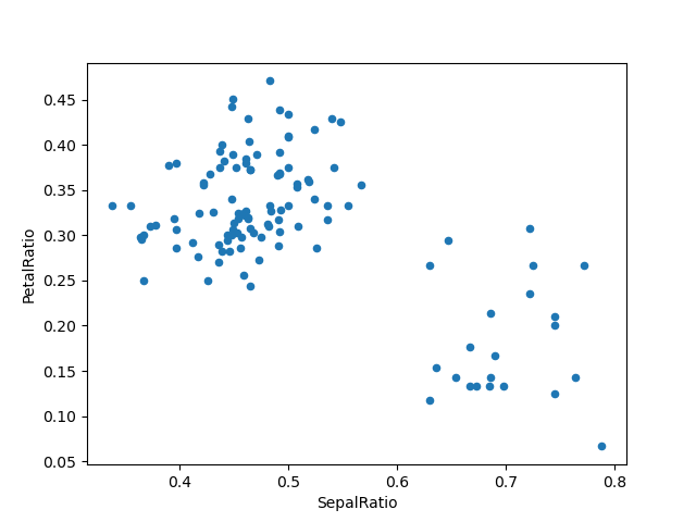
Since a function is passed in, the function is computed on the DataFrame being assigned to. Importantly, this is the DataFrame that’s been filtered to those rows with sepal length greater than 5. The filtering happens first, and then the ratio calculations. This is an example where we didn’t have a reference to the filtered DataFrame available.

The function signature for assign is simply **kwargs. The keys are the column names for the new fields, and the values are either a value to be inserted (for example, a Series or NumPy array), or a function of one argument to be called on the DataFrame. A copy of the original DataFrame is returned, with the new values inserted.

Warning

 

Since the function signature of assign is **kwargs, a dictionary, the order of the new columns in the resulting DataFrame cannot be guaranteed to match the order you pass in. To make things predictable, items are inserted alphabetically (by key) at the end of the DataFrame.

All expressions are computed first, and then assigned. So you can’t refer to another column being assigned in the same call to assign. For example:

In [74]: # Don't do this, bad reference to `C`
        df.assign(C = lambda x: x['A'] + x['B'],
                  D = lambda x: x['A'] + x['C'])
In [2]: # Instead, break it into two assigns
        (df.assign(C = lambda x: x['A'] + x['B'])
           .assign(D = lambda x: x['A'] + x['C']))

Indexing / Selection

The basics of indexing are as follows:

Operation	Syntax	Result
Select column	df[col]	Series
Select row by label	df.loc[label]	Series
Select row by integer location	df.iloc[loc]	Series
Slice rows	df[5:10]	DataFrame
Select rows by boolean vector	df[bool_vec]	DataFrame

Row selection, for example, returns a Series whose index is the columns of the DataFrame:

In [75]: df.loc['b']
Out[75]: 
one              2
bar              2
flag         False
foo            bar
one_trunc        2
Name: b, dtype: object

In [76]: df.iloc[2]
Out[76]: 
one             3
bar             3
flag         True
foo           bar
one_trunc     NaN
Name: c, dtype: object

For a more exhaustive treatment of more sophisticated label-based indexing and slicing, see the section on indexing. We will address the fundamentals of reindexing / conforming to new sets of labels in the section on reindexing.

Data alignment and arithmetic

Data alignment between DataFrame objects automatically align on both the columns and the index (row labels). Again, the resulting object will have the union of the column and row labels.

In [77]: df = pd.DataFrame(np.random.randn(10, 4), columns=['A', 'B', 'C', 'D'])

In [78]: df2 = pd.DataFrame(np.random.randn(7, 3), columns=['A', 'B', 'C'])

In [79]: df + df2
Out[79]: 
        A       B       C   D
0  0.0457 -0.0141  1.3809 NaN
1 -0.9554 -1.5010  0.0372 NaN
2 -0.6627  1.5348 -0.8597 NaN
3 -2.4529  1.2373 -0.1337 NaN
4  1.4145  1.9517 -2.3204 NaN
5 -0.4949 -1.6497 -1.0846 NaN
6 -1.0476 -0.7486 -0.8055 NaN
7     NaN     NaN     NaN NaN
8     NaN     NaN     NaN NaN
9     NaN     NaN     NaN NaN

When doing an operation between DataFrame and Series, the default behavior is to align the Series index on the DataFrame columns, thus broadcasting row-wise. For example:

In [80]: df - df.iloc[0]
Out[80]: 
        A       B       C       D
0  0.0000  0.0000  0.0000  0.0000
1 -1.3593 -0.2487 -0.4534 -1.7547
2  0.2531  0.8297  0.0100 -1.9912
3 -1.3111  0.0543 -1.7249 -1.6205
4  0.5730  1.5007 -0.6761  1.3673
5 -1.7412  0.7820 -1.2416 -2.0531
6 -1.2408 -0.8696 -0.1533  0.0004
7 -0.7439  0.4110 -0.9296 -0.2824
8 -1.1949  1.3207  0.2382 -1.4826
9  2.2938  1.8562  0.7733 -1.4465

In the special case of working with time series data, and the DataFrame index also contains dates, the broadcasting will be column-wise:

In [81]: index = pd.date_range('1/1/2000', periods=8)                           ？？？？？？？？？？？？？？？？？？？？？？？？

In [82]: df = pd.DataFrame(np.random.randn(8, 3), index=index, columns=list('ABC'))

In [83]: df
Out[83]: 
                 A       B       C
2000-01-01 -1.2268  0.7698 -1.2812
2000-01-02 -0.7277 -0.1213 -0.0979
2000-01-03  0.6958  0.3417  0.9597
2000-01-04 -1.1103 -0.6200  0.1497
2000-01-05 -0.7323  0.6877  0.1764
2000-01-06  0.4033 -0.1550  0.3016
2000-01-07 -2.1799 -1.3698 -0.9542
2000-01-08  1.4627 -1.7432 -0.8266

In [84]: type(df['A'])
Out[84]: pandas.core.series.Series

In [85]: df - df['A']
Out[85]: 
            2000-01-01 00:00:00  2000-01-02 00:00:00  2000-01-03 00:00:00  \
2000-01-01                  NaN                  NaN                  NaN   
2000-01-02                  NaN                  NaN                  NaN   
2000-01-03                  NaN                  NaN                  NaN   
2000-01-04                  NaN                  NaN                  NaN   
2000-01-05                  NaN                  NaN                  NaN   
2000-01-06                  NaN                  NaN                  NaN   
2000-01-07                  NaN                  NaN                  NaN   
2000-01-08                  NaN                  NaN                  NaN   

            2000-01-04 00:00:00 ...  2000-01-08 00:00:00   A   B   C  
2000-01-01                  NaN ...                  NaN NaN NaN NaN  
2000-01-02                  NaN ...                  NaN NaN NaN NaN  
2000-01-03                  NaN ...                  NaN NaN NaN NaN  
2000-01-04                  NaN ...                  NaN NaN NaN NaN  
2000-01-05                  NaN ...                  NaN NaN NaN NaN  
2000-01-06                  NaN ...                  NaN NaN NaN NaN  
2000-01-07                  NaN ...                  NaN NaN NaN NaN  
2000-01-08                  NaN ...                  NaN NaN NaN NaN  

[8 rows x 11 columns]

Warning

df - df['A']

is now deprecated and will be removed in a future release. The preferred way to replicate this behavior is

df.sub(df['A'], axis=0)

For explicit control over the matching and broadcasting behavior, see the section on flexible binary operations.

Operations with scalars are just as you would expect:

In [86]: df * 5 + 2
Out[86]: 
                 A       B       C
2000-01-01 -4.1341  5.8490 -4.4062
2000-01-02 -1.6385  1.3935  1.5106
2000-01-03  5.4789  3.7087  6.7986
2000-01-04 -3.5517 -1.0999  2.7487
2000-01-05 -1.6617  5.4387  2.8822
2000-01-06  4.0165  1.2252  3.5081
2000-01-07 -8.8993 -4.8492 -2.7710
2000-01-08  9.3135 -6.7158 -2.1330

In [87]: 1 / df
Out[87]: 
                 A       B        C
2000-01-01 -0.8151  1.2990  -0.7805
2000-01-02 -1.3742 -8.2436 -10.2163
2000-01-03  1.4372  2.9262   1.0420
2000-01-04 -0.9006 -1.6130   6.6779
2000-01-05 -1.3655  1.4540   5.6675
2000-01-06  2.4795 -6.4537   3.3154
2000-01-07 -0.4587 -0.7300  -1.0480
2000-01-08  0.6837 -0.5737  -1.2098

In [88]: df ** 4
Out[88]: 
                  A       B           C
2000-01-01   2.2653  0.3512  2.6948e+00
2000-01-02   0.2804  0.0002  9.1796e-05
2000-01-03   0.2344  0.0136  8.4838e-01
2000-01-04   1.5199  0.1477  5.0286e-04
2000-01-05   0.2876  0.2237  9.6924e-04
2000-01-06   0.0265  0.0006  8.2769e-03
2000-01-07  22.5795  3.5212  8.2903e-01
2000-01-08   4.5774  9.2332  4.6683e-01

Boolean operators work as well:

In [89]: df1 = pd.DataFrame({'a' : [1, 0, 1], 'b' : [0, 1, 1] }, dtype=bool)

In [90]: df2 = pd.DataFrame({'a' : [0, 1, 1], 'b' : [1, 1, 0] }, dtype=bool)

In [91]: df1 & df2   #与
Out[91]: 
       a      b
0  False  False
1  False   True
2   True  False

In [92]: df1 | df2   #或
Out[92]: 
      a     b
0  True  True
1  True  True
2  True  True

In [93]: df1 ^ df2    #异或
Out[93]: 
       a      b
0   True   True
1   True  False
2  False   True

In [94]: -df1    #非
Out[94]: 
       a      b
0  False   True
1   True  False
2  False  False

Transposing

To transpose, access the T attribute (also the transpose function), similar to an ndarray:

# only show the first 5 rows
In [95]: df[:5].T
Out[95]: 
   2000-01-01  2000-01-02  2000-01-03  2000-01-04  2000-01-05
A     -1.2268     -0.7277      0.6958     -1.1103     -0.7323
B      0.7698     -0.1213      0.3417     -0.6200      0.6877
C     -1.2812     -0.0979      0.9597      0.1497      0.1764

置换 

转置,访问 T 属性(也 转置 功能), 类似于一个ndarray:

# only show the first 5 rows
In [95]: df[:5].T
Out[95]: 
   2000-01-01  2000-01-02  2000-01-03  2000-01-04  2000-01-05
A     -1.2268     -0.7277      0.6958     -1.1103     -0.7323
B      0.7698     -0.1213      0.3417     -0.6200      0.6877
C     -1.2812     -0.0979      0.9597      0.1497      0.1764

DataFrame NumPy函数的互用性 

Elementwise NumPy所有日志、exp√,…)和各种其他NumPy功能 可以用于DataFrame上没有问题,假设数据是数字:

In [96]: np.exp(df)
Out[96]: 
                 A       B       C
2000-01-01  0.2932  2.1593  0.2777
2000-01-02  0.4830  0.8858  0.9068
2000-01-03  2.0053  1.4074  2.6110
2000-01-04  0.3294  0.5380  1.1615
2000-01-05  0.4808  1.9892  1.1930
2000-01-06  1.4968  0.8565  1.3521
2000-01-07  0.1131  0.2541  0.3851
2000-01-08  4.3176  0.1750  0.4375

In [97]: np.asarray(df)
Out[97]: 
array([[-1.2268,  0.7698, -1.2812],
       [-0.7277, -0.1213, -0.0979],
       [ 0.6958,  0.3417,  0.9597],
       [-1.1103, -0.62  ,  0.1497],
       [-0.7323,  0.6877,  0.1764],
       [ 0.4033, -0.155 ,  0.3016],
       [-2.1799, -1.3698, -0.9542],
       [ 1.4627, -1.7432, -0.8266]])

点方法DataFrame实现矩阵乘法:

In [98]: df.T.dot(df)
Out[98]: 
         A       B       C
A  11.3419 -0.0598  3.0080
B  -0.0598  6.5206  2.0833
C   3.0080  2.0833  4.3105

同样,点方法实现点系列产品:

In [99]: s1 = pd.Series(np.arange(5,10))

In [100]: s1.dot(s1)
Out[100]: 255

DataFrame并不打算ndarray作为替代 语义索引的地方有很大的不同从一个矩阵。

控制台显示 

非常大的DataFrames将被截断在控制台显示它们。 你也可以使用 信息() 。 (我在这里读的CSV版本 棒球 数据集的 plyr R包):

In [101]: baseball = pd.read_csv('data/baseball.csv')

In [102]: print(baseball)
       id     player  year  stint  ...   hbp   sh   sf  gidp
0   88641  womacto01  2006      2  ...   0.0  3.0  0.0   0.0
1   88643  schilcu01  2006      1  ...   0.0  0.0  0.0   0.0
..    ...        ...   ...    ...  ...   ...  ...  ...   ...
98  89533   aloumo01  2007      1  ...   2.0  0.0  3.0  13.0
99  89534  alomasa02  2007      1  ...   0.0  0.0  0.0   0.0

[100 rows x 23 columns]

In [103]: baseball.info()
<class 'pandas.core.frame.DataFrame'>
RangeIndex: 100 entries, 0 to 99
Data columns (total 23 columns):
id        100 non-null int64
player    100 non-null object
year      100 non-null int64
stint     100 non-null int64
team      100 non-null object
lg        100 non-null object
g         100 non-null int64
ab        100 non-null int64
r         100 non-null int64
h         100 non-null int64
X2b       100 non-null int64
X3b       100 non-null int64
hr        100 non-null int64
rbi       100 non-null float64
sb        100 non-null float64
cs        100 non-null float64
bb        100 non-null int64
so        100 non-null float64
ibb       100 non-null float64
hbp       100 non-null float64
sh        100 non-null float64
sf        100 non-null float64
gidp      100 non-null float64
dtypes: float64(9), int64(11), object(3)
memory usage: 18.0+ KB

然而,使用 to_string 将返回一个字符串表示的吗 DataFrame以表格形式,尽管它并不总是适合控制台宽度:

In [104]: print(baseball.iloc[-20:, :12].to_string())
       id     player  year  stint team  lg    g   ab   r    h  X2b  X3b
80  89474  finlest01  2007      1  COL  NL   43   94   9   17    3    0
81  89480  embreal01  2007      1  OAK  AL    4    0   0    0    0    0
82  89481  edmonji01  2007      1  SLN  NL  117  365  39   92   15    2
83  89482  easleda01  2007      1  NYN  NL   76  193  24   54    6    0
84  89489  delgaca01  2007      1  NYN  NL  139  538  71  139   30    0
85  89493  cormirh01  2007      1  CIN  NL    6    0   0    0    0    0
86  89494  coninje01  2007      2  NYN  NL   21   41   2    8    2    0
87  89495  coninje01  2007      1  CIN  NL   80  215  23   57   11    1
88  89497  clemero02  2007      1  NYA  AL    2    2   0    1    0    0
89  89498  claytro01  2007      2  BOS  AL    8    6   1    0    0    0
90  89499  claytro01  2007      1  TOR  AL   69  189  23   48   14    0
91  89501  cirilje01  2007      2  ARI  NL   28   40   6    8    4    0
92  89502  cirilje01  2007      1  MIN  AL   50  153  18   40    9    2
93  89521  bondsba01  2007      1  SFN  NL  126  340  75   94   14    0
94  89523  biggicr01  2007      1  HOU  NL  141  517  68  130   31    3
95  89525  benitar01  2007      2  FLO  NL   34    0   0    0    0    0
96  89526  benitar01  2007      1  SFN  NL   19    0   0    0    0    0
97  89530  ausmubr01  2007      1  HOU  NL  117  349  38   82   16    3
98  89533   aloumo01  2007      1  NYN  NL   87  328  51  112   19    1
99  89534  alomasa02  2007      1  NYN  NL    8   22   1    3    1    0

宽DataFrames将打印多个行 默认值:

In [105]: pd.DataFrame(np.random.randn(3, 12))
Out[105]: 
         0         1         2         3         4         5         6   \
0 -0.345352  1.314232  0.690579  0.995761  2.396780  0.014871  3.357427   
1 -2.182937  0.380396  0.084844  0.432390  1.519970 -0.493662  0.600178   
2  0.206053 -0.251905 -2.213588  1.063327  1.266143  0.299368 -0.863838   

         7         8         9         10        11  
0 -0.317441 -1.236269  0.896171 -0.487602 -0.082240  
1  0.274230  0.132885 -0.023688  2.410179  1.450520  
2  0.408204 -1.048089 -0.025747 -0.988387  0.094055  

你可以改变多少打印一行通过设置 display.width 选择:

In [106]: pd.set_option('display.width', 40) # default is 80

In [107]: pd.DataFrame(np.random.randn(3, 12))
Out[107]: 
         0         1         2   \
0  1.262731  1.289997  0.082423   
1  1.126203 -0.977349  1.474071   
2  0.758527  1.729689 -0.964980   

         3         4         5   \
0 -0.055758  0.536580 -0.489682   
1 -0.064034 -1.282782  0.781836   
2 -0.845696 -1.340896  1.846883   

         6         7         8   \
0  0.369374 -0.034571 -2.484478   
1 -1.071357  0.441153  2.353925   
2 -1.328865  1.682706 -1.717693   

         9         10        11  
0 -0.281461  0.030711  0.109121  
1  0.583787  0.221471 -0.744471  
2  0.888782  0.228440  0.901805  

你可以调整的最大单个列的宽度设置 display.max_colwidth

In [108]: datafile={'filename': ['filename_01','filename_02'],
   .....:           'path': ["media/user_name/storage/folder_01/filename_01",
   .....:                    "media/user_name/storage/folder_02/filename_02"]}
   .....: 

In [109]: pd.set_option('display.max_colwidth',30)

In [110]: pd.DataFrame(datafile)
Out[110]: 
      filename  \
0  filename_01   
1  filename_02   

                            path  
0  media/user_name/storage/fo...  
1  media/user_name/storage/fo...  

In [111]: pd.set_option('display.max_colwidth',100)

In [112]: pd.DataFrame(datafile)
Out[112]: 
      filename  \
0  filename_01   
1  filename_02   

                                            path  
0  media/user_name/storage/folder_01/filename_01  
1  media/user_name/storage/folder_02/filename_02  

你也可以禁用这个特性通过 expand_frame_repr 选择。 这将打印表在一块。

DataFrame列属性访问和IPython完成 

如果DataFrame列标签是一个有效的Python变量名,列 像访问属性:

In [113]: df = pd.DataFrame({'foo1' : np.random.randn(5),
   .....:                    'foo2' : np.random.randn(5)})
   .....: 

In [114]: df
Out[114]: 
       foo1      foo2
0  1.171216 -0.858447
1  0.520260  0.306996
2 -1.197071 -0.028665
3 -1.066969  0.384316
4 -0.303421  1.574159

In [115]: df.foo1
Out[115]: 
0    1.171216
1    0.520260
2   -1.197071
3   -1.066969
4   -0.303421
Name: foo1, dtype: float64

列也连接到 IPython 补全机制,这样他们可以tab-completed:

In [5]: df.fo<TAB>
df.foo1  df.foo2

面板 （暂时跳过）

警告 

 

在0.20.0, 面板 弃用和将被删除在吗 未来的版本。 看到的部分 反对面板 。

面板有点不常用,但仍然重要的三维容器 数据。 这个词 面板数据 是 来自计量经济学和部分负责熊猫名字: 锅(el)- da(ta)- s。 3轴的名字是为了给一些语义 意义包括面板数据和描述操作,特别是, 面板数据的计量经济分析。 然而,对于严格的切片的目的 和切割DataFrame对象的集合,你会发现轴名称 稍微随意:

• 项目 :轴0,每一项对应一个DataFrame包含在里面
• major_axis :轴1, 指数 (行)的每一个 DataFrames
• minor_axis :轴2, 列 每个DataFrames的

建设小组工作大约像你期望:

与可选的3 d ndarray轴标签 

In [116]: wp = pd.Panel(np.random.randn(2, 5, 4), items=['Item1', 'Item2'],
   .....:               major_axis=pd.date_range('1/1/2000', periods=5),
   .....:               minor_axis=['A', 'B', 'C', 'D'])
   .....: 

In [117]: wp
Out[117]: 
<class 'pandas.core.panel.Panel'>
Dimensions: 2 (items) x 5 (major_axis) x 4 (minor_axis)
Items axis: Item1 to Item2
Major_axis axis: 2000-01-01 00:00:00 to 2000-01-05 00:00:00
Minor_axis axis: A to D

从DataFrame dict对象 

In [118]: data = {'Item1' : pd.DataFrame(np.random.randn(4, 3)),
   .....:         'Item2' : pd.DataFrame(np.random.randn(4, 2))}
   .....: 

In [119]: pd.Panel(data)
Out[119]: 
<class 'pandas.core.panel.Panel'>
Dimensions: 2 (items) x 4 (major_axis) x 3 (minor_axis)
Items axis: Item1 to Item2
Major_axis axis: 0 to 3
Minor_axis axis: 0 to 2

请注意,关键字的值只需要 可转换到 DataFrame 。 因此,他们可以是任何其他有效的DataFrame作为输入 /以上。

一个有用的工厂方法 Panel.from_dict 一个 字典DataFrames如上所述,以下命名参数:

参数	默认的	描述
相交	假	滴元素的指标不一致
东方	项目	使用 小 使用DataFrames”列小组项目

例如,与上面的建设:

In [120]: pd.Panel.from_dict(data, orient='minor')
Out[120]: 
<class 'pandas.core.panel.Panel'>
Dimensions: 3 (items) x 4 (major_axis) x 2 (minor_axis)
Items axis: 0 to 2
Major_axis axis: 0 to 3
Minor_axis axis: Item1 to Item2

东方是特别有用的混合型DataFrames。 如果你通过的东西 DataFrame对象与混合型列,所有数据会向上抛 dtype =对象 除非你通过 东方= '小' :

In [121]: df = pd.DataFrame({'a': ['foo', 'bar', 'baz'],
   .....:                    'b': np.random.randn(3)})
   .....: 

In [122]: df
Out[122]: 
     a         b
0  foo -0.308853
1  bar -0.681087
2  baz  0.377953

In [123]: data = {'item1': df, 'item2': df}

In [124]: panel = pd.Panel.from_dict(data, orient='minor')

In [125]: panel['a']
Out[125]: 
  item1 item2
0   foo   foo
1   bar   bar
2   baz   baz

In [126]: panel['b']
Out[126]: 
      item1     item2
0 -0.308853 -0.308853
1 -0.681087 -0.681087
2  0.377953  0.377953

In [127]: panel['b'].dtypes
Out[127]: 
item1    float64
item2    float64
dtype: object

请注意 

 

面板,比系列和DataFrame不常用, 已经有点被忽视的feature-wise。 一系列的方法和选择 在面板可用在DataFrame并不可用。

从DataFrame使用 to_panel 方法 

to_panel 将一个DataFrame两级指数转换为面板。

In [128]: midx = pd.MultiIndex(levels=[['one', 'two'], ['x','y']], labels=[[1,1,0,0],[1,0,1,0]])

In [129]: df = pd.DataFrame({'A' : [1, 2, 3, 4], 'B': [5, 6, 7, 8]}, index=midx)

In [130]: df.to_panel()
Out[130]: 
<class 'pandas.core.panel.Panel'>
Dimensions: 2 (items) x 2 (major_axis) x 2 (minor_axis)
Items axis: A to B
Major_axis axis: one to two
Minor_axis axis: x to y

项目选择/添加/删除 

类似DataFrame功能的dict系列,小组就像一个东西 DataFrames:

In [131]: wp['Item1']
Out[131]: 
                   A         B         C         D
2000-01-01  1.588931  0.476720  0.473424 -0.242861
2000-01-02 -0.014805 -0.284319  0.650776 -1.461665
2000-01-03 -1.137707 -0.891060 -0.693921  1.613616
2000-01-04  0.464000  0.227371 -0.496922  0.306389
2000-01-05 -2.290613 -1.134623 -1.561819 -0.260838

In [132]: wp['Item3'] = wp['Item1'] / wp['Item2']

插入和删除的API为DataFrame是一样的。 与 python DataFrame,如果项目是一个有效的标识符,你可以作为一个访问 属性和在IPython tab-complete它。

置换 

一个小组可以重新使用它 转置 方法(不做 复制在默认情况下,除非数据异构):

In [133]: wp.transpose(2, 0, 1)
Out[133]: 
<class 'pandas.core.panel.Panel'>
Dimensions: 4 (items) x 3 (major_axis) x 5 (minor_axis)
Items axis: A to D
Major_axis axis: Item1 to Item3
Minor_axis axis: 2000-01-01 00:00:00 to 2000-01-05 00:00:00

索引/选择 

操作	语法	结果
选择项	wp(项)	DataFrame
片在major_axis标签	wp.major_xs(val)	DataFrame
片在minor_axis标签	wp.minor_xs(val)	DataFrame

例如,使用前面的例子的数据,我们能做的:

In [134]: wp['Item1']
Out[134]: 
                   A         B         C         D
2000-01-01  1.588931  0.476720  0.473424 -0.242861
2000-01-02 -0.014805 -0.284319  0.650776 -1.461665
2000-01-03 -1.137707 -0.891060 -0.693921  1.613616
2000-01-04  0.464000  0.227371 -0.496922  0.306389
2000-01-05 -2.290613 -1.134623 -1.561819 -0.260838

In [135]: wp.major_xs(wp.major_axis[2])
Out[135]: 
      Item1     Item2     Item3
A -1.137707  0.800193 -1.421791
B -0.891060  0.782098 -1.139320
C -0.693921 -1.069094  0.649074
D  1.613616 -1.099248 -1.467927

In [136]: wp.minor_axis
Out[136]: Index(['A', 'B', 'C', 'D'], dtype='object')

In [137]: wp.minor_xs('C')
Out[137]: 
               Item1     Item2     Item3
2000-01-01  0.473424 -0.902937 -0.524316
2000-01-02  0.650776 -1.144073 -0.568824
2000-01-03 -0.693921 -1.069094  0.649074
2000-01-04 -0.496922  0.661084 -0.751678
2000-01-05 -1.561819 -1.056652  1.478083

挤压 

改变一个对象的维数的另一种方法是 挤压 1-len对象,类似 wp(“Item1”)

In [138]: wp.reindex(items=['Item1']).squeeze()
Out[138]: 
                   A         B         C         D
2000-01-01  1.588931  0.476720  0.473424 -0.242861
2000-01-02 -0.014805 -0.284319  0.650776 -1.461665
2000-01-03 -1.137707 -0.891060 -0.693921  1.613616
2000-01-04  0.464000  0.227371 -0.496922  0.306389
2000-01-05 -2.290613 -1.134623 -1.561819 -0.260838

In [139]: wp.reindex(items=['Item1'], minor=['B']).squeeze()
Out[139]: 
2000-01-01    0.476720
2000-01-02   -0.284319
2000-01-03   -0.891060
2000-01-04    0.227371
2000-01-05   -1.134623
Freq: D, Name: B, dtype: float64

转换为DataFrame 

面板可以用2 d表示形式作为分层索引 DataFrame。 看到的部分 分层索引 更多的在这。 转换一个DataFrame面板,使用 to_frame 方法:

In [140]: panel = pd.Panel(np.random.randn(3, 5, 4), items=['one', 'two', 'three'],
   .....:                  major_axis=pd.date_range('1/1/2000', periods=5),
   .....:                  minor_axis=['a', 'b', 'c', 'd'])
   .....: 

In [141]: panel.to_frame()
Out[141]: 
                       one       two     three
major      minor                              
2000-01-01 a      0.493672  1.219492 -1.290493
           b     -2.461467  0.062297  0.787872
           c     -1.553902 -0.110388  1.515707
           d      2.015523 -1.184357 -0.276487
2000-01-02 a     -1.833722 -0.558081 -0.223762
           b      1.771740  0.077849  1.397431
           c     -0.670027  0.629498  1.503874
           d      0.049307 -1.035260 -0.478905
2000-01-03 a     -0.521493 -0.438229 -0.135950
           b     -3.201750  0.503703 -0.730327
           c      0.792716  0.413086 -0.033277
           d      0.146111 -1.139050  0.281151
2000-01-04 a      1.903247  0.660342 -1.298915
           b     -0.747169  0.464794 -2.819487
           c     -0.309038 -0.309337 -0.851985
           d      0.393876 -0.649593 -1.106952
2000-01-05 a      1.861468  0.683758 -0.937731
           b      0.936527 -0.643834 -1.537770
           c      1.255746  0.421287  0.555759
           d     -2.655452  1.032814 -2.277282

反对面板 

在过去的几年里,大熊猫在广度和深度,增加了新功能, 数据类型的支持,和操作例程。 因此,支持高效的索引和功能 例程 系列 , DataFrame 和 面板 导致了越来越分散, 难以理解的代码库。

的三维结构 面板 是更常见的对于许多类型的数据分析, 不是一维的 系列 或二维的 DataFrame。 未来是有道理的 熊猫只专注于这些领域。

通常,一个可以简单地使用一个MultiIndex DataFrame 轻松地处理高维数据。

此外, xarray 包是从头构建,专门为了 支持多维分析就是其中之一 面板 年代主要可变性。 这里是一个链接到xarray panel-transition文档 。

In [142]: p = tm.makePanel()

In [143]: p
Out[143]: 
<class 'pandas.core.panel.Panel'>
Dimensions: 3 (items) x 30 (major_axis) x 4 (minor_axis)
Items axis: ItemA to ItemC
Major_axis axis: 2000-01-03 00:00:00 to 2000-02-11 00:00:00
Minor_axis axis: A to D

转换为一个MultiIndex DataFrame

In [144]: p.to_frame()
Out[144]: 
                     ItemA     ItemB     ItemC
major      minor                              
2000-01-03 A     -0.390201 -1.624062 -0.605044
           B      1.562443  0.483103  0.583129
           C     -1.085663  0.768159 -0.273458
           D      0.136235 -0.021763 -0.700648
2000-01-04 A      1.207122 -0.758514  0.878404
           B      0.763264  0.061495 -0.876690
           C     -1.114738  0.225441 -0.335117
           D      0.886313 -0.047152 -1.166607
2000-01-05 A      0.178690 -0.560859 -0.921485
           B      0.162027  0.240767 -1.919354
           C     -0.058216  0.543294 -0.476268
           D     -1.350722  0.088472 -0.367236
2000-01-06 A     -1.004168 -0.589005 -0.200312
           B     -0.902704  0.782413 -0.572707
           C     -0.486768  0.771931 -1.765602
           D     -0.886348 -0.857435  1.296674
2000-01-07 A     -1.377627 -1.070678  0.522423
           B      1.106010  0.628462 -1.736484
           C      1.685148 -0.968145  0.578223
           D     -1.013316 -2.503786  0.641385
2000-01-10 A      0.499281 -1.681101  0.722511
           B     -0.199234 -0.880627 -1.335113
           C      0.112572 -1.176383  0.242697
           D      1.920906 -1.058041 -0.779432
2000-01-11 A     -1.405256  0.403776 -1.702486
           B      0.458265  0.777575 -1.244471
           C     -1.495309 -3.192716  0.208129
           D     -0.388231 -0.657981  0.602456
2000-01-12 A      0.162565  0.609862 -0.709535
           B      0.491048 -0.779367  0.347339
...                    ...       ...       ...
2000-02-02 C     -0.303961 -0.463752 -0.288962
           D      0.104050  1.116086  0.506445
2000-02-03 A     -2.338595 -0.581967 -0.801820
           B     -0.557697 -0.033731 -0.176382
           C      0.625555 -0.055289  0.875359
           D      0.174068 -0.443915  1.626369
2000-02-04 A     -0.374279 -1.233862 -0.915751
           B      0.381353 -1.108761 -1.970108
           C     -0.059268 -0.360853 -0.614618
           D     -0.439461 -0.200491  0.429518
2000-02-07 A     -2.359958 -3.520876 -0.288156
           B      1.337122 -0.314399 -1.044208
           C      0.249698  0.728197  0.565375
           D     -0.741343  1.092633  0.013910
2000-02-08 A     -1.157886  0.516870 -1.199945
           B     -1.531095 -0.860626 -0.821179
           C      1.103949  1.326768  0.068184
           D     -0.079673 -1.675194 -0.458272
2000-02-09 A     -0.551865  0.343125 -0.072869
           B      1.331458  0.370397 -1.914267
           C     -1.087532  0.208927  0.788871
           D     -0.922875  0.437234 -1.531004
2000-02-10 A      1.592673  2.137827 -1.828740
           B     -0.571329 -1.761442 -0.826439
           C      1.998044  0.292058 -0.280343
           D      0.303638  0.388254 -0.500569
2000-02-11 A      1.559318  0.452429 -1.716981
           B     -0.026671 -0.899454  0.124808
           C     -0.244548 -2.019610  0.931536
           D     -0.917368  0.479630  0.870690

[120 rows x 3 columns]

另外,一个可以转换为一个xarray DataArray 。

In [145]: p.to_xarray()
Out[145]: 
<xarray.DataArray (items: 3, major_axis: 30, minor_axis: 4)>
array([[[-0.390201,  1.562443, -1.085663,  0.136235],
        [ 1.207122,  0.763264, -1.114738,  0.886313],
        ..., 
        [ 1.592673, -0.571329,  1.998044,  0.303638],
        [ 1.559318, -0.026671, -0.244548, -0.917368]],

       [[-1.624062,  0.483103,  0.768159, -0.021763],
        [-0.758514,  0.061495,  0.225441, -0.047152],
        ..., 
        [ 2.137827, -1.761442,  0.292058,  0.388254],
        [ 0.452429, -0.899454, -2.01961 ,  0.47963 ]],

       [[-0.605044,  0.583129, -0.273458, -0.700648],
        [ 0.878404, -0.87669 , -0.335117, -1.166607],
        ..., 
        [-1.82874 , -0.826439, -0.280343, -0.500569],
        [-1.716981,  0.124808,  0.931536,  0.87069 ]]])
Coordinates:
  * items       (items) object 'ItemA' 'ItemB' 'ItemC'
  * major_axis  (major_axis) datetime64[ns] 2000-01-03 2000-01-04 2000-01-05 ...
  * minor_axis  (minor_axis) object 'A' 'B' 'C' 'D'

你可以看到的全部文档 xarray包 。

Panel4D和PanelND(弃用) 

警告 

 

在0.19.0 Panel4D 和 PanelND 弃用和将被删除吗 未来的版本。 推荐的方式来表示这些类型的 n维的数据 xarray包 。 大熊猫提供了一个 to_xarray() 方法来自动化 这种转换。

看到 前一版本的文档 这些对象的文档。

------------------------------------------------------------------------------------

Creating a Series by passing a list of values, letting pandas create a default integer index:

In [4]: s = pd.Series([1,3,5,np.nan,6,8])

In [5]: s
Out[5]: 
0    1.0
1    3.0
2    5.0
3    NaN
4    6.0
5    8.0
dtype: float64

Creating a DataFrame by passing a numpy array, with a datetime index and labeled columns:

In [6]: dates = pd.date_range('20130101', periods=6)

In [7]: dates
Out[7]: 
DatetimeIndex(['2013-01-01', '2013-01-02', '2013-01-03', '2013-01-04',
               '2013-01-05', '2013-01-06'],
              dtype='datetime64[ns]', freq='D')

In [8]: df = pd.DataFrame(np.random.randn(6,4), index=dates, columns=list('ABCD'))

In [9]: df
Out[9]: 
                   A         B         C         D
2013-01-01  0.469112 -0.282863 -1.509059 -1.135632
2013-01-02  1.212112 -0.173215  0.119209 -1.044236
2013-01-03 -0.861849 -2.104569 -0.494929  1.071804
2013-01-04  0.721555 -0.706771 -1.039575  0.271860
2013-01-05 -0.424972  0.567020  0.276232 -1.087401
2013-01-06 -0.673690  0.113648 -1.478427  0.524988

Creating a DataFrame by passing a dict of objects that can be converted to series-like.

In [10]: df2 = pd.DataFrame({ 'A' : 1.,
   ....:                      'B' : pd.Timestamp('20130102'),
   ....:                      'C' : pd.Series(1,index=list(range(4)),dtype='float32'),
   ....:                      'D' : np.array([3] * 4,dtype='int32'),
   ....:                      'E' : pd.Categorical(["test","train","test","train"]),
   ....:                      'F' : 'foo' })
   ....: 

In [11]: df2
Out[11]: 
     A          B    C  D      E    F
0  1.0 2013-01-02  1.0  3   test  foo
1  1.0 2013-01-02  1.0  3  train  foo
2  1.0 2013-01-02  1.0  3   test  foo
3  1.0 2013-01-02  1.0  3  train  foo

Having specific dtypes

In [12]: df2.dtypes
Out[12]: 
A           float64
B    datetime64[ns]
C           float32
D             int32
E          category
F            object
dtype: object

If you’re using IPython, tab completion for column names (as well as public attributes) is automatically enabled. Here’s a subset of the attributes that will be completed:

In [13]: df2.<TAB>
df2.A                  df2.bool
df2.abs                df2.boxplot
df2.add                df2.C
df2.add_prefix         df2.clip
df2.add_suffix         df2.clip_lower
df2.align              df2.clip_upper
df2.all                df2.columns
df2.any                df2.combine
df2.append             df2.combine_first
df2.apply              df2.compound
df2.applymap           df2.consolidate
df2.D

As you can see, the columns A, B, C, and D are automatically tab completed. E is there as well; the rest of the attributes have been truncated for brevity.

Viewing Data

See the Basics section

See the top & bottom rows of the frame

In [14]: df.head()
Out[14]: 
                   A         B         C         D
2013-01-01  0.469112 -0.282863 -1.509059 -1.135632
2013-01-02  1.212112 -0.173215  0.119209 -1.044236
2013-01-03 -0.861849 -2.104569 -0.494929  1.071804
2013-01-04  0.721555 -0.706771 -1.039575  0.271860
2013-01-05 -0.424972  0.567020  0.276232 -1.087401

In [15]: df.tail(3)
Out[15]: 
                   A         B         C         D
2013-01-04  0.721555 -0.706771 -1.039575  0.271860
2013-01-05 -0.424972  0.567020  0.276232 -1.087401
2013-01-06 -0.673690  0.113648 -1.478427  0.524988

Display the index, columns, and the underlying numpy data

In [16]: df.index
Out[16]: 
DatetimeIndex(['2013-01-01', '2013-01-02', '2013-01-03', '2013-01-04',
               '2013-01-05', '2013-01-06'],
              dtype='datetime64[ns]', freq='D')

In [17]: df.columns
Out[17]: Index(['A', 'B', 'C', 'D'], dtype='object')

In [18]: df.values
Out[18]: 
array([[ 0.4691, -0.2829, -1.5091, -1.1356],
       [ 1.2121, -0.1732,  0.1192, -1.0442],
       [-0.8618, -2.1046, -0.4949,  1.0718],
       [ 0.7216, -0.7068, -1.0396,  0.2719],
       [-0.425 ,  0.567 ,  0.2762, -1.0874],
       [-0.6737,  0.1136, -1.4784,  0.525 ]])

Describe shows a quick statistic summary of your data

In [19]: df.describe()
Out[19]: 
              A         B         C         D
count  6.000000  6.000000  6.000000  6.000000
mean   0.073711 -0.431125 -0.687758 -0.233103
std    0.843157  0.922818  0.779887  0.973118
min   -0.861849 -2.104569 -1.509059 -1.135632
25%   -0.611510 -0.600794 -1.368714 -1.076610
50%    0.022070 -0.228039 -0.767252 -0.386188
75%    0.658444  0.041933 -0.034326  0.461706
max    1.212112  0.567020  0.276232  1.071804

Transposing your data

In [20]: df.T
Out[20]: 
   2013-01-01  2013-01-02  2013-01-03  2013-01-04  2013-01-05  2013-01-06
A    0.469112    1.212112   -0.861849    0.721555   -0.424972   -0.673690
B   -0.282863   -0.173215   -2.104569   -0.706771    0.567020    0.113648
C   -1.509059    0.119209   -0.494929   -1.039575    0.276232   -1.478427
D   -1.135632   -1.044236    1.071804    0.271860   -1.087401    0.524988

Sorting by an axis

In [21]: df.sort_index(axis=1, ascending=False)
Out[21]: 
                   D         C         B         A
2013-01-01 -1.135632 -1.509059 -0.282863  0.469112
2013-01-02 -1.044236  0.119209 -0.173215  1.212112
2013-01-03  1.071804 -0.494929 -2.104569 -0.861849
2013-01-04  0.271860 -1.039575 -0.706771  0.721555
2013-01-05 -1.087401  0.276232  0.567020 -0.424972
2013-01-06  0.524988 -1.478427  0.113648 -0.673690

Sorting by values

In [22]: df.sort_values(by='B')
Out[22]: 
                   A         B         C         D
2013-01-03 -0.861849 -2.104569 -0.494929  1.071804
2013-01-04  0.721555 -0.706771 -1.039575  0.271860
2013-01-01  0.469112 -0.282863 -1.509059 -1.135632
2013-01-02  1.212112 -0.173215  0.119209 -1.044236
2013-01-06 -0.673690  0.113648 -1.478427  0.524988
2013-01-05 -0.424972  0.567020  0.276232 -1.087401

Selection

Note

 

While standard Python / Numpy expressions for selecting and setting are intuitive and come in handy for interactive work, for production code, we recommend the optimized pandas data access methods, .at, .iat, .loc,.iloc and .ix.

See the indexing documentation Indexing and Selecting Data and MultiIndex / Advanced Indexing

Getting

Selecting a single column, which yields a Series, equivalent to df.A

In [23]: df['A']
Out[23]: 
2013-01-01    0.469112
2013-01-02    1.212112
2013-01-03   -0.861849
2013-01-04    0.721555
2013-01-05   -0.424972
2013-01-06   -0.673690
Freq: D, Name: A, dtype: float64

Selecting via [], which slices the rows.

In [24]: df[0:3]
Out[24]: 
                   A         B         C         D
2013-01-01  0.469112 -0.282863 -1.509059 -1.135632
2013-01-02  1.212112 -0.173215  0.119209 -1.044236
2013-01-03 -0.861849 -2.104569 -0.494929  1.071804

In [25]: df['20130102':'20130104']
Out[25]: 
                   A         B         C         D
2013-01-02  1.212112 -0.173215  0.119209 -1.044236
2013-01-03 -0.861849 -2.104569 -0.494929  1.071804
2013-01-04  0.721555 -0.706771 -1.039575  0.271860

Selection by Label

See more in Selection by Label

For getting a cross section using a label

In [26]: df.loc[dates[0]]
Out[26]: 
A    0.469112
B   -0.282863
C   -1.509059
D   -1.135632
Name: 2013-01-01 00:00:00, dtype: float64

Selecting on a multi-axis by label

In [27]: df.loc[:,['A','B']]
Out[27]: 
                   A         B
2013-01-01  0.469112 -0.282863
2013-01-02  1.212112 -0.173215
2013-01-03 -0.861849 -2.104569
2013-01-04  0.721555 -0.706771
2013-01-05 -0.424972  0.567020
2013-01-06 -0.673690  0.113648

Showing label slicing, both endpoints are included

In [28]: df.loc['20130102':'20130104',['A','B']]
Out[28]: 
                   A         B
2013-01-02  1.212112 -0.173215
2013-01-03 -0.861849 -2.104569
2013-01-04  0.721555 -0.706771

Reduction in the dimensions of the returned object

In [29]: df.loc['20130102',['A','B']]
Out[29]: 
A    1.212112
B   -0.173215
Name: 2013-01-02 00:00:00, dtype: float64

For getting a scalar value

In [30]: df.loc[dates[0],'A']
Out[30]: 0.46911229990718628

For getting fast access to a scalar (equiv to the prior method)

In [31]: df.at[dates[0],'A']
Out[31]: 0.46911229990718628

Selection by Position

See more in Selection by Position

Select via the position of the passed integers

In [32]: df.iloc[3]
Out[32]: 
A    0.721555
B   -0.706771
C   -1.039575
D    0.271860
Name: 2013-01-04 00:00:00, dtype: float64

By integer slices, acting similar to numpy/python

In [33]: df.iloc[3:5,0:2]
Out[33]: 
                   A         B
2013-01-04  0.721555 -0.706771
2013-01-05 -0.424972  0.567020

By lists of integer position locations, similar to the numpy/python style

In [34]: df.iloc[[1,2,4],[0,2]]
Out[34]: 
                   A         C
2013-01-02  1.212112  0.119209
2013-01-03 -0.861849 -0.494929
2013-01-05 -0.424972  0.276232

For slicing rows explicitly

In [35]: df.iloc[1:3,:]
Out[35]: 
                   A         B         C         D
2013-01-02  1.212112 -0.173215  0.119209 -1.044236
2013-01-03 -0.861849 -2.104569 -0.494929  1.071804

For slicing columns explicitly

In [36]: df.iloc[:,1:3]
Out[36]: 
                   B         C
2013-01-01 -0.282863 -1.509059
2013-01-02 -0.173215  0.119209
2013-01-03 -2.104569 -0.494929
2013-01-04 -0.706771 -1.039575
2013-01-05  0.567020  0.276232
2013-01-06  0.113648 -1.478427

For getting a value explicitly

In [37]: df.iloc[1,1]
Out[37]: -0.17321464905330858

For getting fast access to a scalar (equiv to the prior method)

In [38]: df.iat[1,1]
Out[38]: -0.17321464905330858

Boolean Indexing

Using a single column’s values to select data.

In [39]: df[df.A > 0]
Out[39]: 
                   A         B         C         D
2013-01-01  0.469112 -0.282863 -1.509059 -1.135632
2013-01-02  1.212112 -0.173215  0.119209 -1.044236
2013-01-04  0.721555 -0.706771 -1.039575  0.271860

Selecting values from a DataFrame where a boolean condition is met.

In [40]: df[df > 0]
Out[40]: 
                   A         B         C         D
2013-01-01  0.469112       NaN       NaN       NaN
2013-01-02  1.212112       NaN  0.119209       NaN
2013-01-03       NaN       NaN       NaN  1.071804
2013-01-04  0.721555       NaN       NaN  0.271860
2013-01-05       NaN  0.567020  0.276232       NaN
2013-01-06       NaN  0.113648       NaN  0.524988

Using the isin() method for filtering:

In [41]: df2 = df.copy()

In [42]: df2['E'] = ['one', 'one','two','three','four','three']

In [43]: df2
Out[43]: 
                   A         B         C         D      E
2013-01-01  0.469112 -0.282863 -1.509059 -1.135632    one
2013-01-02  1.212112 -0.173215  0.119209 -1.044236    one
2013-01-03 -0.861849 -2.104569 -0.494929  1.071804    two
2013-01-04  0.721555 -0.706771 -1.039575  0.271860  three
2013-01-05 -0.424972  0.567020  0.276232 -1.087401   four
2013-01-06 -0.673690  0.113648 -1.478427  0.524988  three

In [44]: df2[df2['E'].isin(['two','four'])]
Out[44]: 
                   A         B         C         D     E
2013-01-03 -0.861849 -2.104569 -0.494929  1.071804   two
2013-01-05 -0.424972  0.567020  0.276232 -1.087401  four

Setting

Setting a new column automatically aligns the data by the indexes

In [45]: s1 = pd.Series([1,2,3,4,5,6], index=pd.date_range('20130102', periods=6))

In [46]: s1
Out[46]: 
2013-01-02    1
2013-01-03    2
2013-01-04    3
2013-01-05    4
2013-01-06    5
2013-01-07    6
Freq: D, dtype: int64

In [47]: df['F'] = s1

Setting values by label

In [48]: df.at[dates[0],'A'] = 0

Setting values by position

In [49]: df.iat[0,1] = 0

Setting by assigning with a numpy array

In [50]: df.loc[:,'D'] = np.array([5] * len(df))

The result of the prior setting operations

In [51]: df
Out[51]: 
                   A         B         C  D    F
2013-01-01  0.000000  0.000000 -1.509059  5  NaN
2013-01-02  1.212112 -0.173215  0.119209  5  1.0
2013-01-03 -0.861849 -2.104569 -0.494929  5  2.0
2013-01-04  0.721555 -0.706771 -1.039575  5  3.0
2013-01-05 -0.424972  0.567020  0.276232  5  4.0
2013-01-06 -0.673690  0.113648 -1.478427  5  5.0

A where operation with setting.

In [52]: df2 = df.copy()

In [53]: df2[df2 > 0] = -df2

In [54]: df2
Out[54]: 
                   A         B         C  D    F
2013-01-01  0.000000  0.000000 -1.509059 -5  NaN
2013-01-02 -1.212112 -0.173215 -0.119209 -5 -1.0
2013-01-03 -0.861849 -2.104569 -0.494929 -5 -2.0
2013-01-04 -0.721555 -0.706771 -1.039575 -5 -3.0
2013-01-05 -0.424972 -0.567020 -0.276232 -5 -4.0
2013-01-06 -0.673690 -0.113648 -1.478427 -5 -5.0

Missing Data

pandas primarily uses the value np.nan to represent missing data. It is by default not included in computations. See the Missing Data section

Reindexing allows you to change/add/delete the index on a specified axis. This returns a copy of the data.

In [55]: df1 = df.reindex(index=dates[0:4], columns=list(df.columns) + ['E'])

In [56]: df1.loc[dates[0]:dates[1],'E'] = 1

In [57]: df1
Out[57]: 
                   A         B         C  D    F    E
2013-01-01  0.000000  0.000000 -1.509059  5  NaN  1.0
2013-01-02  1.212112 -0.173215  0.119209  5  1.0  1.0
2013-01-03 -0.861849 -2.104569 -0.494929  5  2.0  NaN
2013-01-04  0.721555 -0.706771 -1.039575  5  3.0  NaN

To drop any rows that have missing data.

In [58]: df1.dropna(how='any')
Out[58]: 
                   A         B         C  D    F    E
2013-01-02  1.212112 -0.173215  0.119209  5  1.0  1.0

Filling missing data

In [59]: df1.fillna(value=5)
Out[59]: 
                   A         B         C  D    F    E
2013-01-01  0.000000  0.000000 -1.509059  5  5.0  1.0
2013-01-02  1.212112 -0.173215  0.119209  5  1.0  1.0
2013-01-03 -0.861849 -2.104569 -0.494929  5  2.0  5.0
2013-01-04  0.721555 -0.706771 -1.039575  5  3.0  5.0

To get the boolean mask where values are nan

In [60]: pd.isna(df1)
Out[60]: 
                A      B      C      D      F      E
2013-01-01  False  False  False  False   True  False
2013-01-02  False  False  False  False  False  False
2013-01-03  False  False  False  False  False   True
2013-01-04  False  False  False  False  False   True

Operations

See the Basic section on Binary Ops

Stats

Operations in general exclude missing data.

Performing a descriptive statistic

In [61]: df.mean()
Out[61]: 
A   -0.004474
B   -0.383981
C   -0.687758
D    5.000000
F    3.000000
dtype: float64

Same operation on the other axis

In [62]: df.mean(1)
Out[62]: 
2013-01-01    0.872735
2013-01-02    1.431621
2013-01-03    0.707731
2013-01-04    1.395042
2013-01-05    1.883656
2013-01-06    1.592306
Freq: D, dtype: float64

Operating with objects that have different dimensionality and need alignment. In addition, pandas automatically broadcasts along the specified dimension.

In [63]: s = pd.Series([1,3,5,np.nan,6,8], index=dates).shift(2)

In [64]: s
Out[64]: 
2013-01-01    NaN
2013-01-02    NaN
2013-01-03    1.0
2013-01-04    3.0
2013-01-05    5.0
2013-01-06    NaN
Freq: D, dtype: float64

In [65]: df.sub(s, axis='index')
Out[65]: 
                   A         B         C    D    F
2013-01-01       NaN       NaN       NaN  NaN  NaN
2013-01-02       NaN       NaN       NaN  NaN  NaN
2013-01-03 -1.861849 -3.104569 -1.494929  4.0  1.0
2013-01-04 -2.278445 -3.706771 -4.039575  2.0  0.0
2013-01-05 -5.424972 -4.432980 -4.723768  0.0 -1.0
2013-01-06       NaN       NaN       NaN  NaN  NaN

Apply

Applying functions to the data

In [66]: df.apply(np.cumsum)
Out[66]: 
                   A         B         C   D     F
2013-01-01  0.000000  0.000000 -1.509059   5   NaN
2013-01-02  1.212112 -0.173215 -1.389850  10   1.0
2013-01-03  0.350263 -2.277784 -1.884779  15   3.0
2013-01-04  1.071818 -2.984555 -2.924354  20   6.0
2013-01-05  0.646846 -2.417535 -2.648122  25  10.0
2013-01-06 -0.026844 -2.303886 -4.126549  30  15.0

In [67]: df.apply(lambda x: x.max() - x.min())
Out[67]: 
A    2.073961
B    2.671590
C    1.785291
D    0.000000
F    4.000000
dtype: float64

Histogramming

See more at Histogramming and Discretization

In [68]: s = pd.Series(np.random.randint(0, 7, size=10))

In [69]: s
Out[69]: 
0    4
1    2
2    1
3    2
4    6
5    4
6    4
7    6
8    4
9    4
dtype: int64

In [70]: s.value_counts()
Out[70]: 
4    5
6    2
2    2
1    1
dtype: int64

String Methods

Series is equipped with a set of string processing methods in the str attribute that make it easy to operate on each element of the array, as in the code snippet below. Note that pattern-matching in str generally uses regular expressions by default (and in some cases always uses them). See more at Vectorized String Methods.

In [71]: s = pd.Series(['A', 'B', 'C', 'Aaba', 'Baca', np.nan, 'CABA', 'dog', 'cat'])

In [72]: s.str.lower()
Out[72]: 
0       a
1       b
2       c
3    aaba
4    baca
5     NaN
6    caba
7     dog
8     cat
dtype: object

Merge

Concat

pandas provides various facilities for easily combining together Series, DataFrame, and Panel objects with various kinds of set logic for the indexes and relational algebra functionality in the case of join / merge-type operations.

See the Merging section

Concatenating pandas objects together with concat():

In [73]: df = pd.DataFrame(np.random.randn(10, 4))

In [74]: df
Out[74]: 
          0         1         2         3
0 -0.548702  1.467327 -1.015962 -0.483075
1  1.637550 -1.217659 -0.291519 -1.745505
2 -0.263952  0.991460 -0.919069  0.266046
3 -0.709661  1.669052  1.037882 -1.705775
4 -0.919854 -0.042379  1.247642 -0.009920
5  0.290213  0.495767  0.362949  1.548106
6 -1.131345 -0.089329  0.337863 -0.945867
7 -0.932132  1.956030  0.017587 -0.016692
8 -0.575247  0.254161 -1.143704  0.215897
9  1.193555 -0.077118 -0.408530 -0.862495

# break it into pieces
In [75]: pieces = [df[:3], df[3:7], df[7:]]

In [76]: pd.concat(pieces)
Out[76]: 
          0         1         2         3
0 -0.548702  1.467327 -1.015962 -0.483075
1  1.637550 -1.217659 -0.291519 -1.745505
2 -0.263952  0.991460 -0.919069  0.266046
3 -0.709661  1.669052  1.037882 -1.705775
4 -0.919854 -0.042379  1.247642 -0.009920
5  0.290213  0.495767  0.362949  1.548106
6 -1.131345 -0.089329  0.337863 -0.945867
7 -0.932132  1.956030  0.017587 -0.016692
8 -0.575247  0.254161 -1.143704  0.215897
9  1.193555 -0.077118 -0.408530 -0.862495

Join

SQL style merges. See the Database style joining

In [77]: left = pd.DataFrame({'key': ['foo', 'foo'], 'lval': [1, 2]})

In [78]: right = pd.DataFrame({'key': ['foo', 'foo'], 'rval': [4, 5]})

In [79]: left
Out[79]: 
   key  lval
0  foo     1
1  foo     2

In [80]: right
Out[80]: 
   key  rval
0  foo     4
1  foo     5

In [81]: pd.merge(left, right, on='key')
Out[81]: 
   key  lval  rval
0  foo     1     4
1  foo     1     5
2  foo     2     4
3  foo     2     5

Another example that can be given is:

In [82]: left = pd.DataFrame({'key': ['foo', 'bar'], 'lval': [1, 2]})

In [83]: right = pd.DataFrame({'key': ['foo', 'bar'], 'rval': [4, 5]})

In [84]: left
Out[84]: 
   key  lval
0  foo     1
1  bar     2

In [85]: right
Out[85]: 
   key  rval
0  foo     4
1  bar     5

In [86]: pd.merge(left, right, on='key')
Out[86]: 
   key  lval  rval
0  foo     1     4
1  bar     2     5

Append

Append rows to a dataframe. See the Appending

In [87]: df = pd.DataFrame(np.random.randn(8, 4), columns=['A','B','C','D'])

In [88]: df
Out[88]: 
          A         B         C         D
0  1.346061  1.511763  1.627081 -0.990582
1 -0.441652  1.211526  0.268520  0.024580
2 -1.577585  0.396823 -0.105381 -0.532532
3  1.453749  1.208843 -0.080952 -0.264610
4 -0.727965 -0.589346  0.339969 -0.693205
5 -0.339355  0.593616  0.884345  1.591431
6  0.141809  0.220390  0.435589  0.192451
7 -0.096701  0.803351  1.715071 -0.708758

In [89]: s = df.iloc[3]

In [90]: df.append(s, ignore_index=True)
Out[90]: 
          A         B         C         D
0  1.346061  1.511763  1.627081 -0.990582
1 -0.441652  1.211526  0.268520  0.024580
2 -1.577585  0.396823 -0.105381 -0.532532
3  1.453749  1.208843 -0.080952 -0.264610
4 -0.727965 -0.589346  0.339969 -0.693205
5 -0.339355  0.593616  0.884345  1.591431
6  0.141809  0.220390  0.435589  0.192451
7 -0.096701  0.803351  1.715071 -0.708758
8  1.453749  1.208843 -0.080952 -0.264610

Grouping

By “group by” we are referring to a process involving one or more of the following steps

• Splitting the data into groups based on some criteria
• Applying a function to each group independently
• Combining the results into a data structure

See the Grouping section

In [91]: df = pd.DataFrame({'A' : ['foo', 'bar', 'foo', 'bar',
   ....:                           'foo', 'bar', 'foo', 'foo'],
   ....:                    'B' : ['one', 'one', 'two', 'three',
   ....:                           'two', 'two', 'one', 'three'],
   ....:                    'C' : np.random.randn(8),
   ....:                    'D' : np.random.randn(8)})
   ....: 

In [92]: df
Out[92]: 
     A      B         C         D
0  foo    one -1.202872 -0.055224
1  bar    one -1.814470  2.395985
2  foo    two  1.018601  1.552825
3  bar  three -0.595447  0.166599
4  foo    two  1.395433  0.047609
5  bar    two -0.392670 -0.136473
6  foo    one  0.007207 -0.561757
7  foo  three  1.928123 -1.623033

Grouping and then applying a function sum to the resulting groups.

In [93]: df.groupby('A').sum()
Out[93]: 
            C        D
A                     
bar -2.802588  2.42611
foo  3.146492 -0.63958

Grouping by multiple columns forms a hierarchical index, which we then apply the function.

In [94]: df.groupby(['A','B']).sum()
Out[94]: 
                  C         D
A   B                        
bar one   -1.814470  2.395985
    three -0.595447  0.166599
    two   -0.392670 -0.136473
foo one   -1.195665 -0.616981
    three  1.928123 -1.623033
    two    2.414034  1.600434

Reshaping

See the sections on Hierarchical Indexing and Reshaping.

Stack

In [95]: tuples = list(zip(*[['bar', 'bar', 'baz', 'baz',
   ....:                      'foo', 'foo', 'qux', 'qux'],
   ....:                     ['one', 'two', 'one', 'two',
   ....:                      'one', 'two', 'one', 'two']]))
   ....: 

In [96]: index = pd.MultiIndex.from_tuples(tuples, names=['first', 'second'])

In [97]: df = pd.DataFrame(np.random.randn(8, 2), index=index, columns=['A', 'B'])

In [98]: df2 = df[:4]

In [99]: df2
Out[99]: 
                     A         B
first second                    
bar   one     0.029399 -0.542108
      two     0.282696 -0.087302
baz   one    -1.575170  1.771208
      two     0.816482  1.100230

The stack() method “compresses” a level in the DataFrame’s columns.

In [100]: stacked = df2.stack()

In [101]: stacked
Out[101]: 
first  second   
bar    one     A    0.029399
               B   -0.542108
       two     A    0.282696
               B   -0.087302
baz    one     A   -1.575170
               B    1.771208
       two     A    0.816482
               B    1.100230
dtype: float64

With a “stacked” DataFrame or Series (having a MultiIndex as the index), the inverse operation of stack() isunstack(), which by default unstacks the last levelIn [102]: stacked.unstack()Out[102]: 

                     A         B
first second                    
bar   one     0.029399 -0.542108
      two     0.282696 -0.087302
baz   one    -1.575170  1.771208
      two     0.816482  1.100230

In [103]: stacked.unstack(1)
Out[103]: 
second        one       two
first                      
bar   A  0.029399  0.282696
      B -0.542108 -0.087302
baz   A -1.575170  0.816482
      B  1.771208  1.100230

In [104]: stacked.unstack(0)
Out[104]: 
first          bar       baz
second                      
one    A  0.029399 -1.575170
       B -0.542108  1.771208
two    A  0.282696  0.816482
       B -0.087302  1.100230
------------------------------------------------------------------------------------------------------------------------------
此处以下，以后再看。

 

Pivot Tables

See the section on Pivot Tables.

In [105]: df = pd.DataFrame({'A' : ['one', 'one', 'two', 'three'] * 3,
   .....:                    'B' : ['A', 'B', 'C'] * 4,
   .....:                    'C' : ['foo', 'foo', 'foo', 'bar', 'bar', 'bar'] * 2,
   .....:                    'D' : np.random.randn(12),
   .....:                    'E' : np.random.randn(12)})
   .....: 

In [106]: df
Out[106]: 
        A  B    C         D         E
0     one  A  foo  1.418757 -0.179666
1     one  B  foo -1.879024  1.291836
2     two  C  foo  0.536826 -0.009614
3   three  A  bar  1.006160  0.392149
4     one  B  bar -0.029716  0.264599
5     one  C  bar -1.146178 -0.057409
6     two  A  foo  0.100900 -1.425638
7   three  B  foo -1.035018  1.024098
8     one  C  foo  0.314665 -0.106062
9     one  A  bar -0.773723  1.824375
10    two  B  bar -1.170653  0.595974
11  three  C  bar  0.648740  1.167115

We can produce pivot tables from this data very easily:

In [107]: pd.pivot_table(df, values='D', index=['A', 'B'], columns=['C'])
Out[107]: 
C             bar       foo
A     B                    
one   A -0.773723  1.418757
      B -0.029716 -1.879024
      C -1.146178  0.314665
three A  1.006160       NaN
      B       NaN -1.035018
      C  0.648740       NaN
two   A       NaN  0.100900
      B -1.170653       NaN
      C       NaN  0.536826

Time Series

pandas has simple, powerful, and efficient functionality for performing resampling operations during frequency conversion (e.g., converting secondly data into 5-minutely data). This is extremely common in, but not limited to, financial applications. See the Time Series section

In [108]: rng = pd.date_range('1/1/2012', periods=100, freq='S')

In [109]: ts = pd.Series(np.random.randint(0, 500, len(rng)), index=rng)

In [110]: ts.resample('5Min').sum()
Out[110]: 
2012-01-01    25083
Freq: 5T, dtype: int64

Time zone representation

In [111]: rng = pd.date_range('3/6/2012 00:00', periods=5, freq='D')

In [112]: ts = pd.Series(np.random.randn(len(rng)), rng)

In [113]: ts
Out[113]: 
2012-03-06    0.464000
2012-03-07    0.227371
2012-03-08   -0.496922
2012-03-09    0.306389
2012-03-10   -2.290613
Freq: D, dtype: float64

In [114]: ts_utc = ts.tz_localize('UTC')

In [115]: ts_utc
Out[115]: 
2012-03-06 00:00:00+00:00    0.464000
2012-03-07 00:00:00+00:00    0.227371
2012-03-08 00:00:00+00:00   -0.496922
2012-03-09 00:00:00+00:00    0.306389
2012-03-10 00:00:00+00:00   -2.290613
Freq: D, dtype: float64

Convert to another time zone

In [116]: ts_utc.tz_convert('US/Eastern')
Out[116]: 
2012-03-05 19:00:00-05:00    0.464000
2012-03-06 19:00:00-05:00    0.227371
2012-03-07 19:00:00-05:00   -0.496922
2012-03-08 19:00:00-05:00    0.306389
2012-03-09 19:00:00-05:00   -2.290613
Freq: D, dtype: float64

Converting between time span representations

In [117]: rng = pd.date_range('1/1/2012', periods=5, freq='M')

In [118]: ts = pd.Series(np.random.randn(len(rng)), index=rng)

In [119]: ts
Out[119]: 
2012-01-31   -1.134623
2012-02-29   -1.561819
2012-03-31   -0.260838
2012-04-30    0.281957
2012-05-31    1.523962
Freq: M, dtype: float64

In [120]: ps = ts.to_period()

In [121]: ps
Out[121]: 
2012-01   -1.134623
2012-02   -1.561819
2012-03   -0.260838
2012-04    0.281957
2012-05    1.523962
Freq: M, dtype: float64

In [122]: ps.to_timestamp()
Out[122]: 
2012-01-01   -1.134623
2012-02-01   -1.561819
2012-03-01   -0.260838
2012-04-01    0.281957
2012-05-01    1.523962
Freq: MS, dtype: float64

Converting between period and timestamp enables some convenient arithmetic functions to be used. In the following example, we convert a quarterly frequency with year ending in November to 9am of the end of the month following the quarter end:

In [123]: prng = pd.period_range('1990Q1', '2000Q4', freq='Q-NOV')

In [124]: ts = pd.Series(np.random.randn(len(prng)), prng)

In [125]: ts.index = (prng.asfreq('M', 'e') + 1).asfreq('H', 's') + 9

In [126]: ts.head()
Out[126]: 
1990-03-01 09:00   -0.902937
1990-06-01 09:00    0.068159
1990-09-01 09:00   -0.057873
1990-12-01 09:00   -0.368204
1991-03-01 09:00   -1.144073
Freq: H, dtype: float64

Categoricals

pandas can include categorical data in a DataFrame. For full docs, see the categorical introduction and the API documentation.

In [127]: df = pd.DataFrame({"id":[1,2,3,4,5,6], "raw_grade":['a', 'b', 'b', 'a', 'a', 'e']})

Convert the raw grades to a categorical data type.

In [128]: df["grade"] = df["raw_grade"].astype("category")

In [129]: df["grade"]
Out[129]: 
0    a
1    b
2    b
3    a
4    a
5    e
Name: grade, dtype: category
Categories (3, object): [a, b, e]

Rename the categories to more meaningful names (assigning to Series.cat.categories is inplace!)

In [130]: df["grade"].cat.categories = ["very good", "good", "very bad"]

Reorder the categories and simultaneously add the missing categories (methods under Series .cat return a new Series per default).

In [131]: df["grade"] = df["grade"].cat.set_categories(["very bad", "bad", "medium", "good", "very good"])

In [132]: df["grade"]
Out[132]: 
0    very good
1         good
2         good
3    very good
4    very good
5     very bad
Name: grade, dtype: category
Categories (5, object): [very bad, bad, medium, good, very good]

Sorting is per order in the categories, not lexical order.

In [133]: df.sort_values(by="grade")
Out[133]: 
   id raw_grade      grade
5   6         e   very bad
1   2         b       good
2   3         b       good
0   1         a  very good
3   4         a  very good
4   5         a  very good

Grouping by a categorical column shows also empty categories.

In [134]: df.groupby("grade").size()
Out[134]: 
grade
very bad     1
bad          0
medium       0
good         2
very good    3
dtype: int64

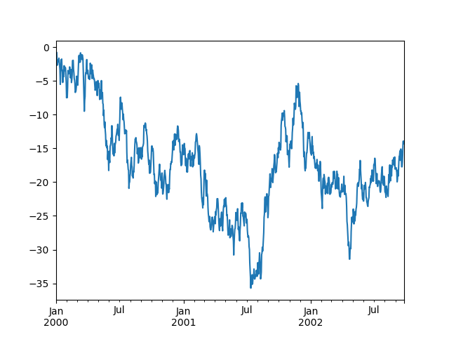
Plotting

Plotting docs.

In [135]: ts = pd.Series(np.random.randn(1000), index=pd.date_range('1/1/2000', periods=1000))

In [136]: ts = ts.cumsum()

In [137]: ts.plot()
Out[137]: <matplotlib.axes._subplots.AxesSubplot at 0x1122ad630>

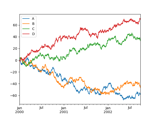
On DataFrame, plot() is a convenience to plot all of the columns with labels:

In [138]: df = pd.DataFrame(np.random.randn(1000, 4), index=ts.index,
   .....:                   columns=['A', 'B', 'C', 'D'])
   .....: 

In [139]: df = df.cumsum()

In [140]: plt.figure(); df.plot(); plt.legend(loc='best')
Out[140]: <matplotlib.legend.Legend at 0x115033cf8>

Getting Data In/Out

CSV

Writing to a csv file

In [141]: df.to_csv('foo.csv')

Reading from a csv file

In [142]: pd.read_csv('foo.csv')
Out[142]: 
     Unnamed: 0          A          B         C          D
0    2000-01-01   0.266457  -0.399641 -0.219582   1.186860
1    2000-01-02  -1.170732  -0.345873  1.653061  -0.282953
2    2000-01-03  -1.734933   0.530468  2.060811  -0.515536
3    2000-01-04  -1.555121   1.452620  0.239859  -1.156896
4    2000-01-05   0.578117   0.511371  0.103552  -2.428202
5    2000-01-06   0.478344   0.449933 -0.741620  -1.962409
6    2000-01-07   1.235339  -0.091757 -1.543861  -1.084753
..          ...        ...        ...       ...        ...
993  2002-09-20 -10.628548  -9.153563 -7.883146  28.313940
994  2002-09-21 -10.390377  -8.727491 -6.399645  30.914107
995  2002-09-22  -8.985362  -8.485624 -4.669462  31.367740
996  2002-09-23  -9.558560  -8.781216 -4.499815  30.518439
997  2002-09-24  -9.902058  -9.340490 -4.386639  30.105593
998  2002-09-25 -10.216020  -9.480682 -3.933802  29.758560
999  2002-09-26 -11.856774 -10.671012 -3.216025  29.369368

[1000 rows x 5 columns]

HDF5

Reading and writing to HDFStores

Writing to a HDF5 Store

In [143]: df.to_hdf('foo.h5','df')

Reading from a HDF5 Store

In [144]: pd.read_hdf('foo.h5','df')
Out[144]: 
                    A          B         C          D
2000-01-01   0.266457  -0.399641 -0.219582   1.186860
2000-01-02  -1.170732  -0.345873  1.653061  -0.282953
2000-01-03  -1.734933   0.530468  2.060811  -0.515536
2000-01-04  -1.555121   1.452620  0.239859  -1.156896
2000-01-05   0.578117   0.511371  0.103552  -2.428202
2000-01-06   0.478344   0.449933 -0.741620  -1.962409
2000-01-07   1.235339  -0.091757 -1.543861  -1.084753
...               ...        ...       ...        ...
2002-09-20 -10.628548  -9.153563 -7.883146  28.313940
2002-09-21 -10.390377  -8.727491 -6.399645  30.914107
2002-09-22  -8.985362  -8.485624 -4.669462  31.367740
2002-09-23  -9.558560  -8.781216 -4.499815  30.518439
2002-09-24  -9.902058  -9.340490 -4.386639  30.105593
2002-09-25 -10.216020  -9.480682 -3.933802  29.758560
2002-09-26 -11.856774 -10.671012 -3.216025  29.369368

[1000 rows x 4 columns]

Excel

Reading and writing to MS Excel

Writing to an excel file

In [145]: df.to_excel('foo.xlsx', sheet_name='Sheet1')

Reading from an excel file

In [146]: pd.read_excel('foo.xlsx', 'Sheet1', index_col=None, na_values=['NA'])
Out[146]: 
                    A          B         C          D
2000-01-01   0.266457  -0.399641 -0.219582   1.186860
2000-01-02  -1.170732  -0.345873  1.653061  -0.282953
2000-01-03  -1.734933   0.530468  2.060811  -0.515536
2000-01-04  -1.555121   1.452620  0.239859  -1.156896
2000-01-05   0.578117   0.511371  0.103552  -2.428202
2000-01-06   0.478344   0.449933 -0.741620  -1.962409
2000-01-07   1.235339  -0.091757 -1.543861  -1.084753
...               ...        ...       ...        ...
2002-09-20 -10.628548  -9.153563 -7.883146  28.313940
2002-09-21 -10.390377  -8.727491 -6.399645  30.914107
2002-09-22  -8.985362  -8.485624 -4.669462  31.367740
2002-09-23  -9.558560  -8.781216 -4.499815  30.518439
2002-09-24  -9.902058  -9.340490 -4.386639  30.105593
2002-09-25 -10.216020  -9.480682 -3.933802  29.758560
2002-09-26 -11.856774 -10.671012 -3.216025  29.369368

[1000 rows x 4 columns]

Gotchas

If you are trying an operation and you see an exception like:

>>> if pd.Series([False, True, False]):
    print("I was true")
Traceback
    ...
ValueError: The truth value of an array is ambiguous. Use a.empty, a.any() or a.all().

See Comparisons for an explanation and what to do.

See Gotchas as well.