『高性能模型』深度可分离卷积和MobileNet_v1

TensorFlow预训练模型：mobilenet_v1.md

一、深度可分离卷积

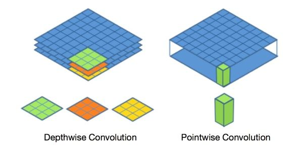
标准的卷积过程可以看上图，一个2×2的卷积核在卷积时，对应图像区域中的所有通道均被同时考虑，问题在于，为什么一定要同时考虑图像区域和通道？我们为什么不能把通道和空间区域分开考虑？

深度可分离卷积提出了一种新的思路：对于不同的输入channel采取不同的卷积核进行卷积，它将普通的卷积操作分解为两个过程。

卷积过程

假设有 $N\times H\times W \times C$ 的输入，同时有 $k$ 个 $3\times3$ 的卷积。如果设置 $pad=1$ 且 $stride=1$ ，那么普通卷积输出为 $N\times H\times W \times k$ 。

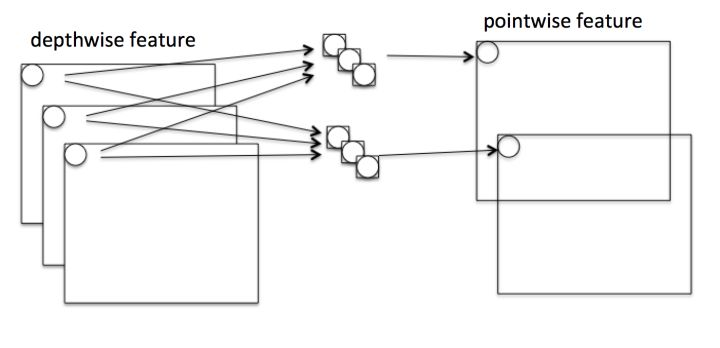
Depthwise 过程

Depthwise是指将 $N\times H\times W \times C$ 的输入分为 $group=C$ 组，然后每一组做 $3\times3$ 卷积。这样相当于收集了每个Channel的空间特征，即Depthwise特征。

Pointwise 过程

Pointwise是指对 $N\times H\times W \times C$ 的输入做 $k$ 个普通的 $1\times1$ 卷积。这样相当于收集了每个点的特征，即Pointwise特征。Depthwise+Pointwise最终输出也是 $N\times H\times W \times k$ 。

二、优势与创新

Depthwise+Pointwise可以近似看作一个卷积层：

普通卷积：3x3 Conv+BN+ReLU
Mobilenet卷积：3x3 Depthwise Conv+BN+ReLU 和 1x1 Pointwise Conv+BN+ReLU

计算加速

参数量降低

假设输入通道数为3，要求输出通道数为256，两种做法：

1.直接接一个3×3×256的卷积核，参数量为：3×3×3×256 = 6,912

2.DW操作，分两步完成，参数量为：3×3×3 + 3×1×1×256 = 795（3个特征层*（3*3的卷积核）），卷积深度参数通常取为1

乘法运算次数降低

对比一下不同卷积的乘法次数：

普通卷积计算量为： $H\times W \times C\times k \times 3\times 3$
Depthwise计算量为： $H\times W \times C \times 3\times 3$
Pointwise计算量为： $H\times W\times C\times k$

通过Depthwise+Pointwise的拆分，相当于将普通卷积的计算量压缩为：

$\frac{depthwise+pointwise}{conv}=\frac{H\times W \times C \times 3\times 3 + H\times W\times C\times k}{H\times W \times C\times k \times 3\times 3}=\frac{1}{k} +\frac{1}{3\times 3}$

通道区域分离

深度可分离卷积将以往普通卷积操作同时考虑通道和区域改变（卷积先只考虑区域，然后再考虑通道），实现了通道和区域的分离。

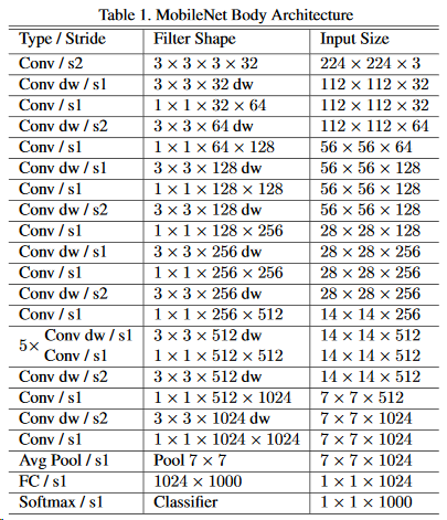
三、Mobilenet v1

Mobilenet v1利用深度可分离卷积进行加速，其架构如下，

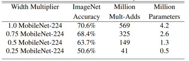
还可以对所有卷积层 $kernel$ 数量统一乘以缩小因子 $\alpha$ （其中 $\alpha\in(0,1]，典型值为1，0.75，0.5和0.25$ ）以压缩网络。这样Depthwise+Pointwise总计算量可以进一降低为：

$H\times W \times \alpha C \times 3\times 3 + H\times W\times \alpha C\times \alpha k$

当然，压缩网络计算量肯定是有代价的。下图展示了 $\alpha$ 不同时Mobilenet v1在ImageNet上的性能。可以看到即使 $\alpha=0.5$ 时Mobilenet v1在ImageNet上依然有63.7%的准确度。

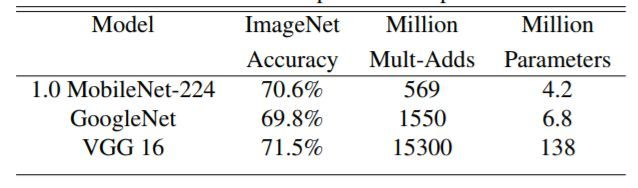
下图展示Mobilenet v1 $\alpha=1.0$ 与GoogleNet和VGG16的在输入分辨率 $224\times 224$ 情况下，准确度差距非常小，但是计算量和参数量都小很多。同时原文也给出了以Mobilenet v1提取特征的SSD/Faster R-CNN在COCO数据集上的性能。

结构实现一探

在实现代码中（链接见本文开头），作者使用具名元组存储了网络结构信息，

Conv = namedtuple('Conv', ['kernel', 'stride', 'depth'])
DepthSepConv = namedtuple('DepthSepConv', ['kernel', 'stride', 'depth'])

# MOBILENETV1_CONV_DEFS specifies the MobileNet body
MOBILENETV1_CONV_DEFS = [
    Conv(kernel=[3, 3], stride=2, depth=32),
    DepthSepConv(kernel=[3, 3], stride=1, depth=64),
    DepthSepConv(kernel=[3, 3], stride=2, depth=128),
    DepthSepConv(kernel=[3, 3], stride=1, depth=128),
    DepthSepConv(kernel=[3, 3], stride=2, depth=256),
    DepthSepConv(kernel=[3, 3], stride=1, depth=256),
    DepthSepConv(kernel=[3, 3], stride=2, depth=512),
    DepthSepConv(kernel=[3, 3], stride=1, depth=512),
    DepthSepConv(kernel=[3, 3], stride=1, depth=512),
    DepthSepConv(kernel=[3, 3], stride=1, depth=512),
    DepthSepConv(kernel=[3, 3], stride=1, depth=512),
    DepthSepConv(kernel=[3, 3], stride=1, depth=512),
    DepthSepConv(kernel=[3, 3], stride=2, depth=1024),
    DepthSepConv(kernel=[3, 3], stride=1, depth=1024)
]

然后，在生成结构中迭代这个具名元组列表，根据信息生成网路结构，这仅仅给出深度可分离层的实现部分，

elif isinstance(conv_def, DepthSepConv):
      end_point = end_point_base + '_depthwise'

      # By passing filters=None
      # separable_conv2d produces only a depthwise convolution layer
      if use_explicit_padding:
        net = _fixed_padding(net, conv_def.kernel, layer_rate)
      net = slim.separable_conv2d(net, None, conv_def.kernel,  # <---Depthwise
                                  depth_multiplier=1,
                                  stride=layer_stride,
                                  rate=layer_rate,
                                  scope=end_point)

      end_points[end_point] = net
      if end_point == final_endpoint:
        return net, end_points
      end_point = end_point_base + '_pointwise'
      net = slim.conv2d(net, depth(conv_def.depth), [1, 1],  # <---Pointwise
                        stride=1,
                        scope=end_point)

四、相关框架实现

TensorFlow 分步执行

顺便一提，tf的实现可以接收rate参数，即可以采用空洞卷积的方式进行操作。

1、depthwise_conv2d 分离卷积部分

我们定义一张4*4的双通道图片

import tensorflow as tf

img1 = tf.constant(value=[[[[1],[2],[3],[4]],
                           [[1],[2],[3],[4]],
                           [[1],[2],[3],[4]],
                           [[1],[2],[3],[4]]]],dtype=tf.float32)

img2 = tf.constant(value=[[[[1],[1],[1],[1]],
                           [[1],[1],[1],[1]],
                           [[1],[1],[1],[1]],
                           [[1],[1],[1],[1]]]],dtype=tf.float32)

img = tf.concat(values=[img1,img2],axis=3)

img

<tf.Tensor 'concat_1:0' shape=(1, 4, 4, 2) dtype=float32>

使用3*3的卷积核，输入channel为2，输出channel为2（卷积核数目为2），

filter1 = tf.constant(value=0, shape=[3,3,1,1],dtype=tf.float32)
filter2 = tf.constant(value=1, shape=[3,3,1,1],dtype=tf.float32)
filter3 = tf.constant(value=2, shape=[3,3,1,1],dtype=tf.float32)
filter4 = tf.constant(value=3, shape=[3,3,1,1],dtype=tf.float32)
filter_out1 = tf.concat(values=[filter1,filter2],axis=2)
filter_out2 = tf.concat(values=[filter3,filter4],axis=2)
filter = tf.concat(values=[filter_out1,filter_out2],axis=3)

filter

<tf.Tensor 'concat_4:0' shape=(3, 3, 2, 2) dtype=float32>

同时执行卷积操作，和深度可分离卷积操作，

out_img_conv = tf.nn.conv2d(input=img, filter=filter, 
                            strides=[1,1,1,1], padding='VALID')
out_img_depthwise = tf.nn.depthwise_conv2d(input=img, 
                                           filter=filter, strides=[1,1,1,1], 
　　　　　　　　　　　　　　　　　　　　　　　　　　rate=[1,1], padding='VALID')

with tf.Session() as sess:
    res1 = sess.run(out_img_conv)
    res2 = sess.run(out_img_depthwise)
print(res1, '\n', res1.shape)
print(res2, '\n', res2.shape)

[[[[  9.  63.]
   [  9.  81.]]

  [[  9.  63.]
   [  9.  81.]]]] 
 (1, 2, 2, 2)  # 《----------


[[[[  0.  36.   9.  27.]
   [  0.  54.   9.  27.]]

  [[  0.  36.   9.  27.]
   [  0.  54.   9.  27.]]]] 
 (1, 2, 2, 4)# 《----------

对比输出shape，depthwise_conv2d输出的channel数目为in_channel * 卷积核数目，每一个卷积核对应通道都会对对应的channel进行一次卷积，所以输出通道数更多，

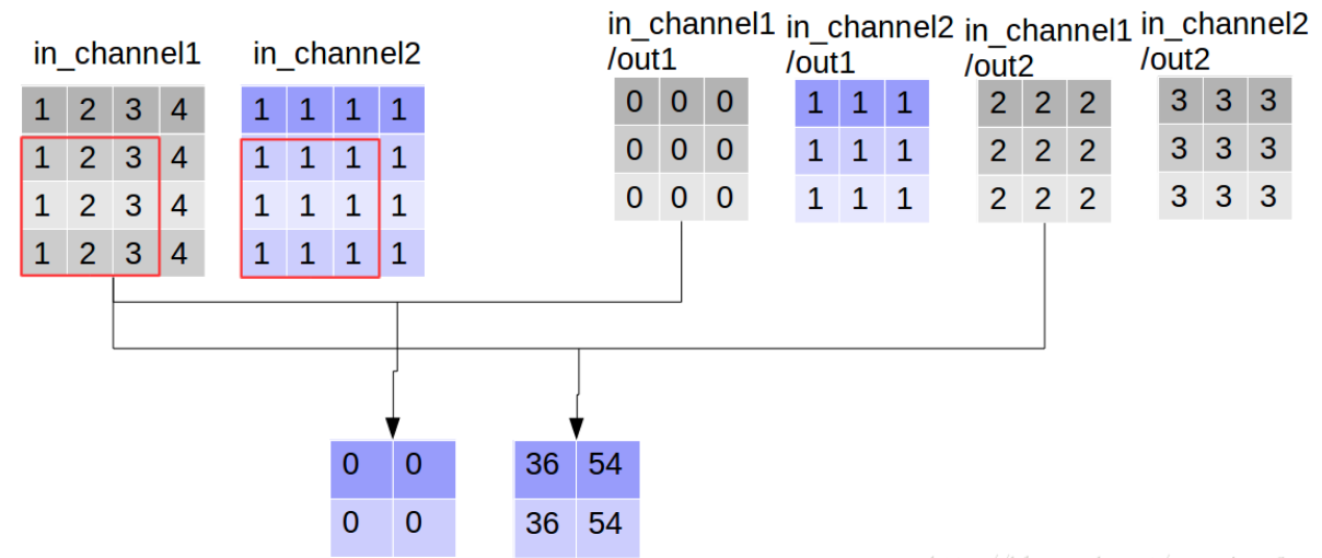
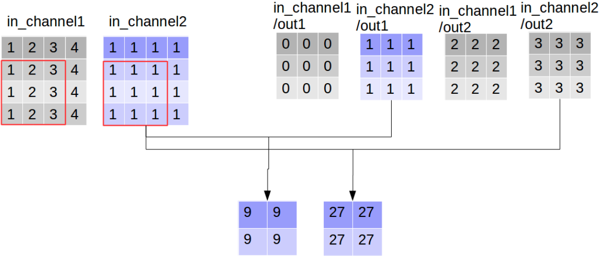
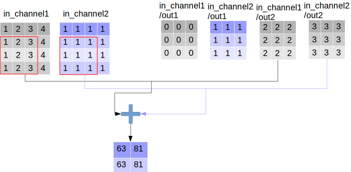
看到这里大家可能会误解深度可分离卷积的输出通道数大于普通卷积，其实这只是“分离”部分，后面还有组合的步骤，而普通卷积只不过直接完成了组合：通过对应点相加，将四个卷积中间结果合并为卷积核个数（这里是2）

2、合并特征

合并过程如下，可分离卷积中的合并过程变成可学习的了，使用一个1*1的普通卷积进行特征合并，

point_filter = tf.constant(value=1, shape=[1,1,4,4],dtype=tf.float32)
out_img_s = tf.nn.conv2d(input=out_img_depthwise, filter=point_filter, strides=[1,1,1,1], padding='VALID')
with tf.Session() as sess:
    res3 = sess.run(out_img_s)
print(res3, '\n', res3.shape)

[[[[ 72.  72.  72.  72.]
   [ 90.  90.  90.  90.]]

  [[ 72.  72.  72.  72.]
   [ 90.  90.  90.  90.]]]] 
 (1, 2, 2, 4)

TensorFlow 一步执行

out_img_se = tf.nn.separable_conv2d(input=img, 
                                    depthwise_filter=filter, 
                                    pointwise_filter=point_filter, 
                                    strides=[1,1,1,1], rate=[1,1], padding='VALID')

with tf.Session() as sess:
    print(sess.run(out_img_se))

[[[[ 72. 72. 72. 72.]
[ 90. 90. 90. 90.]]

[[ 72. 72. 72. 72.]
[ 90. 90. 90. 90.]]]]
(1, 2, 2, 4)

slim 库API介绍

def separable_convolution2d(
    inputs,
    num_outputs,
    kernel_size,
    depth_multiplier=1,
    stride=1,
    padding='SAME',
    data_format=DATA_FORMAT_NHWC,
    rate=1,
    activation_fn=nn.relu,
    normalizer_fn=None,
    normalizer_params=None,
    weights_initializer=initializers.xavier_initializer(),
    pointwise_initializer=None,
    weights_regularizer=None,
    biases_initializer=init_ops.zeros_initializer(),
    biases_regularizer=None,
    reuse=None,
    variables_collections=None,
    outputs_collections=None,
    trainable=True,
    scope=None):

  """一个2维的可分离卷积，可以选择是否增加BN层。
  这个操作首先执行逐通道的卷积（每个通道分别执行卷积），创建一个称为depthwise_weights的变量。如果num_outputs
不为空，它将增加一个pointwise的卷积（混合通道间的信息），创建一个称为pointwise_weights的变量。如果
normalizer_fn为空，它将给结果加上一个偏置，并且创建一个为biases的变量，如果不为空，那么归一化函数将被调用。
最后再调用一个激活函数然后得到最终的结果。

  Args:
    inputs: 一个形状为[batch_size, height, width, channels]的tensor
    num_outputs: pointwise 卷积的卷积核个数，如果为空，将跳过pointwise卷积的步骤.
    kernel_size: 卷积核的尺寸：[kernel_height, kernel_width]，如果两个的值相同，则可以为一个整数。
    depth_multiplier: 卷积乘子，即每个输入通道经过卷积后的输出通道数。总共的输出通道数将为：
num_filters_in * depth_multiplier。
    stride:卷积步长，[stride_height, stride_width],如果两个值相同的话，为一个整数值。
    padding:  填充方式，'VALID' 或者 'SAME'.
    data_format:数据格式， `NHWC` (默认) 和 `NCHW` 
    rate: 空洞卷积的膨胀率：[rate_height, rate_width],如果两个值相同的话，可以为整数值。如果这两个值
任意一个大于1，那么stride的值必须为1.     
    activation_fn: 激活函数，默认为ReLU。如果设置为None，将跳过。
    normalizer_fn: 归一化函数，用来替代biase。如果归一化函数不为空，那么biases_initializer
和biases_regularizer将被忽略。 biases将不会被创建。如果设为None，将不会有归一化。
    normalizer_params: 归一化函数的参数。
    weights_initializer: depthwise卷积的权重初始化器
    pointwise_initializer: pointwise卷积的权重初始化器。如果设为None，将使用weights_initializer。
    weights_regularizer: (可选)权重正则化器。
    biases_initializer: 偏置初始化器，如果为None，将跳过偏置。
    biases_regularizer: (可选)偏置正则化器。
    reuse: 网络层和它的变量是否可以被重用，为了重用，网络层的scope必须被提供。
    variables_collections: (可选)所有变量的collection列表，或者是一个关键字为变量值为collection的字典。
    outputs_collections: 输出被添加的collection.
    trainable: 变量是否可以被训练
    scope: (可选)变量的命名空间。
  Returns:
    代表这个操作的输出的一个tensor"""

posted @ 2018-09-29 20:20 叠加态的猫阅读(24479) 评论(3) 编辑收藏举报

叠加态的猫