A-Softmax的总结及与L-Softmax的对比——SphereFace

A-Softmax的总结及与L-Softmax的对比——SphereFace

\(\quad\)【引言】SphereFace在MegaFace数据集上识别率在2017年排名第一，用的A-Softmax Loss有着清晰的几何定义，能在比较小的数据集上达到不错的效果。这个是他们总结成果的论文：SphereFace: Deep Hypersphere Embedding for Face Recognition。我对论文做一个小的总结。

1. A-Softmax的推导

回顾一下二分类下的Softmax后验概率，即：

\[\begin{split} p_1 = \frac{\exp({W}_1^Tx+b_1)}{\exp({W}_1^Tx+b_1)+\exp({W}_2^Tx+b_2)} \cr p_2 = \frac{\exp({W}_2^Tx+b_2)}{\exp({W}_1^Tx+b_1)+\exp({W}_2^Tx+b_2)} \cr \end{split} \tag{1.1} \]

\(\quad\)显然决策的分界在当\(p_1 = p_2\)时，所以决策界面是\((W_1-W_2)x+b_1-b_2=0\)。我们可以将\(W_i^Tx+b_i\)写成\(\|W_i^T\|\cdot\|x\|\cos(\theta_i)+b_i\)，其中\(\theta_i\)是\(W_i\)与\(x\)的夹角，如对\(W_i\)归一化且设偏置\(b_i\)为零（\(\|W_i\|=1\)，\(b_i=0\)），那么当\(p_1 = p_2\)时，我们有\(\cos(\theta_1)-\cos(\theta_2)=0\)。从这里可以看到，如里一个输入的数据特征\(x_i\)属于\(y_i\)类，那么\(\theta_{yi}\)应该比其它所有类的角度都要小，也就是说在向量空间中\(W_{yi}\)要更靠近\(x_i\)。
\(\quad\)我们用的是Softmax Loss，对于输入\(x_i\)，Softmax Loss \(L_i\)定义以下：

\[\begin{split} L_i &= -\log(\frac{\exp(W_{yi}^Tx_i+b_{yi})}{\sum_j\exp(W_{j}^Tx_i+b_{j})}) \cr &= -\log(\frac{\exp(\|W_{yi}^T\|·\|x_i\|\cos(\theta_{yi,i})+b_{yi})}{\sum_j\exp(\|W_{j}^T\|·\|x_i\|\cos(\theta_{j,i})+b_{j})}) \cr \end{split} \tag{1.2} \]

式\((1.2)\)中的\(j\in[1,K]\)，其中\(K\)类别的总数。上面我们限制了一些条件：\(\|W_i\|=1\)，\(b_i=0\)，由这些条件，可以得到修正的损失函数（也就是论文中所以说的modified softmax loss）：

\[L_{modified} = \frac{1}{N}\sum_i-\log(\frac{\exp(\|x_i\|\cos(\theta_{yi,i}))}{\sum_j\exp(\|x_i\|\cos(\theta_{j,i}))}) \tag{1.3} \]

\(\quad\)在二分类问题中，当\(\cos(\theta_1)>\cos(\theta_2)\)时，可以确定属于类别1，但分类1与分类2的决策面是同一分，说明分类1与分类2之间的间隔(margin)相当小，直观上的感觉就是分类不明显。如果要让分类1与分类2有一个明显的间隔，可以做两个决策面，对于类别1的决策平面为：\(\cos(m\theta_1)=\cos(\theta_2)\)，对于类别2的策平面为：\(\cos(\theta_1)=\cos(m\theta_2)\)，其中\(m\geq2,m\in N\)。\(m\)是整数的目的是为了方便计算，因为可以利用倍角公式，\(m\geq2\)说明与该分类的最大夹角要比其它类的小小夹角还要小\(m\)倍。如果\(m=1\),那么类别1与类别2的决策平面是同一个平面，如果\(m\geq2\)v，那么类别1与类别2的有两个决策平面，相隔多大将会在性质中说明。从上述的说明与\(L_{modified}\)可以直接得到A-Softmax Loss：

\[L_{ang} = \frac{1}{N}\sum_i-\log(\frac{\exp(\|x_i\|\cos(m\theta_{yi,i}))}{\exp(\|x_i\|\cos(m\theta_{yi,i}))+\sum_{j\neq y_i}\exp(\|x_i\|\cos(\theta_{j,i}))}) \tag{1.4} \]

其中\(\theta_{yi,i}\in[0, \frac{\pi}{m}]\)，因为\(\theta_{yi,i}\)在这个范围之外可可能会使得\(m\theta_{y_i,i}>\theta_{j,i},j\neq y_i\)（这样就不属于分类\(y_i\)了），但\(\cos(m\theta_1)>\cos(\theta_2)\)仍可能成立，而我们Loss方程用的还是\(\cos(\theta)\)。为了避免这个问题，可以重新设计一个函数来替代\(\cos(m\theta_{y_i,i})\)，定义\(\psi(\theta_{y_i,i})=(-1)^k\cos(m\theta_{y_i,i})-2k\)，其中\(\theta_{y_i,i}\in[\frac{k\pi}{m},\frac{(k+1)\pi}{m}]\)，\(且k\in[1,k]\)。这个函数的定义可以使得\(\psi\)随\(\theta_{y_i,i}\)单调递减，如果\(m\theta_{y_i,i}>\theta_{j,i},j\neq y_i\), 那么必有\(\psi(\theta_{y_i,i})<\cos(\theta_{j,i})\)，反而亦然，这样可以避免上述的问题，所以有：

\[L_{ang} = \frac{1}{N}\sum_i-\log(\frac{\exp(\|x_i\|\psi(\theta_{yi,i}))}{\exp(\|x_i\|\psi(\theta_{yi,i}))+\sum_{j\neq y_i}\exp(\|x_i\|\cos(\theta_{j,i}))}) \tag{1.5} \]

\(\quad\)对于以上三种二分类问题的Loss（多分类是差不多的情况）的决策面，可以总结如下表：

\[\begin{array}{|c|l|} \hline \text{Loss Funtion} & \text{Decision Boundary} \\ \hline \text{Softmax Loss} & (W_1-W_2)x+b_1-b_2=0\\ \hline \text{Modified Softmax Loss} & \|x\|(\cos\theta_1-\cos\theta_2)=0 \\ \hline \text{A-Softmax Loss} & Class1: \|x\|(\cos m\theta_1-\cos\theta_2)=0 \\ & Class2: \|x\|(\cos \theta_1-\cos m\theta_2)=0\\ \hline \end{array} \]

\(\quad\)论文中还给出了这三种不同Loss的几何意义，可以看到的是普通的softmax（Euclidean Margin Loss）是在欧氏空间中分开的，它映射到欧氏空间中是不同的区域的空间，决策面是一个在欧氏空间中的平面，可以分隔不同的类别。Modified Softmax Loss与A-Softmax Loss的不同之处在于两个不同类的决策平面是同一个，不像A-Softmax Loss，有两个分隔的决策平面且决策平面分隔的大小还是与\(m\)的大小成正相关，如下图所示。

2. A-Softmax Loss的性质

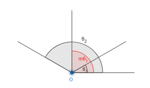
性质1：A-Softmax Loss定义了一个大角度间隔的学习方法，\(m\)越大这个间隔的角度也就越大，相应区域流形的大小就越小，这就导致了训练的任务也越困难。
这个性质是相当容易理解的，如图1所示：这个间隔的角度为\((m-1)\theta_1\)，所以\(m\)越大，则间隔的角度就越小；同时\(m\theta_1<\pi\)，当所以\(m\)越大，则相应的区域流形\(\theta_1\)就越小。

图1：性质1的示意图

定义1：\(m_{min}\)被定义为当\(m>m_{min}\)时有类内间的最大角度特征距离小于类间的最小角度特征距离。
性质2：在二分类问题中：\(m_{min}>2+\sqrt{3}\)，有多分类问题中：\(m_{min}\geq 3\)。
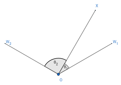
证明：1.对于二分类问题，设\(W_1\)、\(W_2\)分别是类别1与类别2的权重，\(W_1\)与\(W_2\)之间的夹角是\(\theta_{12}\)，输入的特征为\(x\)，那么权重与输入特征之间的夹角就决定了输入的特征属于那个类别，不失一般性地可以认为输入的特征性于类别1，则有\(m\theta_1<\theta_2\)。当\(x\)在\(\theta_{12}\)之间时，如图2所示，可以由\(m\theta_1=\theta_2\)求出这时\(\theta_1\)的最大值为\(\theta_{max1}^{in}=\frac{\theta_{12}}{m+1}\)。

图2：$x$在$\theta_{12}$之间时的示意图

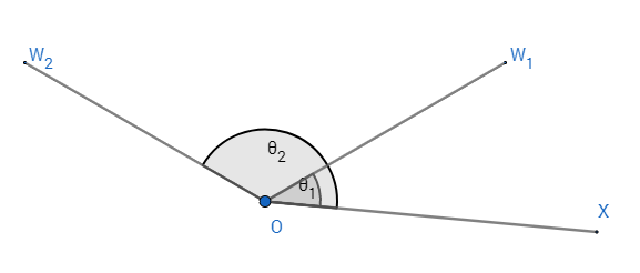
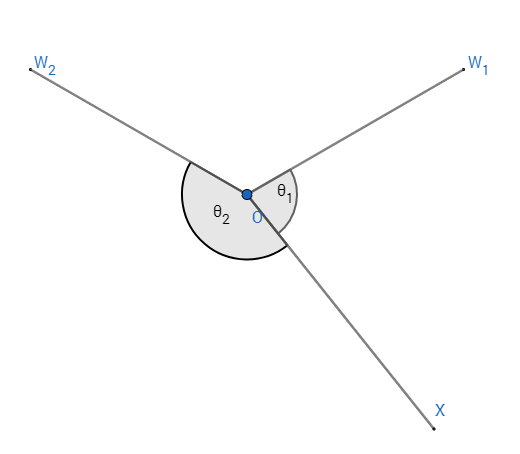
当\(x\)在\(\theta_{12}\)之外时，第一种情况是当\(\theta_{12} \leq \frac{m-1}{m}\pi\)，如图3所示，可以由\(m\theta_1=\theta_2\)求出这时\(\theta_1\)的最大值为\(\theta_{max1}^{out}=\frac{\theta_{12}}{m-1}\)，还有一种情况就是当\(\theta_1\)与\(\theta_2\)不是同一侧时，\(\theta_{12} < \frac{m-1}{m}\pi\)，如图4所示，可以得到：\(\theta_{max1}^{out}=\frac{2\pi-\theta_{12}}{m+1}\)。

图3：$x$在$\theta_{12}$之外时的示意图

图4：$x$在$\theta_{12}$之外时的示意图

无论是上述中的第一种情况还是第二种情况，类间的最小角度特征距离如图5所示情况中的\(\theta_{inter}\),所以有：\(\theta_{inter}=(m-1)\theta_1=\frac{m-1}{m+1}\theta_{12}\)。

图5：最小的类间距离示意图

以上的分析可以总结为以下方程：

\[\begin{split} \frac{\theta_{12}}{m-1} + \frac{\theta_{12}}{m+1} \leq \frac{m-1}{m+1}\theta_{12}, \theta_{12} \leq \frac{m-1}{m}\pi \cr \frac{2\pi - \theta_{12}}{m-1} + \frac{\theta_{12}}{m+1} \leq \frac{m-1}{m+1}\theta_{12}, \theta_{12} > \frac{m-1}{m}\pi \cr \end{split} \tag{2.1} \]

解上述不等式可以行到\(m_{min} \geq 2+\sqrt{3}\)。
2.对于\(K\)类(\(K\geq 3\))问题，设\(\theta_i^{i+1}\)是权重\(W_i\)与\(W_{i+1}\)的夹角，显然最好的情况是\(W_i\)是均匀分布的，所以有\(\theta_i^{i+1}=\frac{2\pi}{K}\)。对于类内的最大距离与类间的小距离有以下方程：

\[\frac{\theta_{i}^{i+1}}{m+1} +　\frac{\theta_{i-1}^{i}}{m+1} < min\{\frac{(m-1)\theta_{i}^{i+1}}{m+1}, \frac{(m-1)\theta_{i-1}^{i}}{m+1}\} \tag{2.2} \]

可以解得\(m_{min} \geq 3\)。综合上面对\(m_{min}\)的讨论，论文中取了\(m=4\)。

3. A-Softmax的几何意义

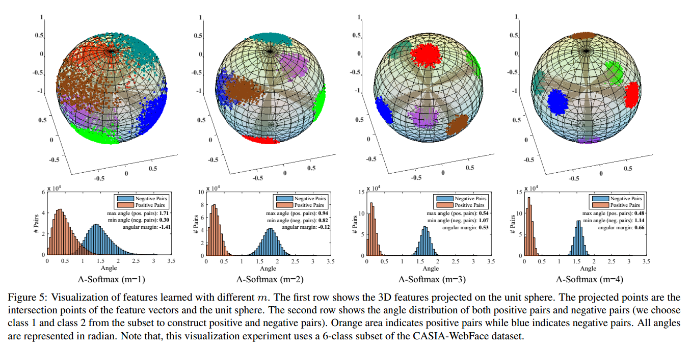
个人认为A-Softmax是基于一个假设：不同的类位于一个单位超球表面的不同区域。从上面也可以知道它的几何意义是权重所代表的在单位超球表面的点，在训练的过程中，同一类的输入映射到表面上会慢慢地向中心点（这里的中心点大部分时候和权重的意义相当）聚集，而到不同类的权重（或者中心点）慢慢地分散开来。\(m\)的大小是控制同一类点聚集的程度，从而控制了不同类之间的距离。从图6可以看到，不同的\(m\)对映射分布的影响（作者画的图真好看，也不知道作者是怎么画出来的）。

图6：不同的$m$对映射分布的影响

4. 源码解读

\(\quad\)作者用Caffe实现了A-Softmax，可以参考这个wy1iu/SphereFace，来解读其中的一些细节。在实际的编程中，不需要直接实现式\((1.4)\)中的\(L_{ang}\)，可以在SoftmaxOut层前面加一层\(MarginInnerProduct\)，这个文件sphereface_model.prototxt的最后如下面引用所示，可以看到作者是加多了一层。具体的C++代码在margin_inner_product_layer.cpp。

############### A-Softmax Loss ##############
layer {
  name: "fc6"
  type: "MarginInnerProduct"
  bottom: "fc5"
  bottom: "label"
  top: "fc6"
  top: "lambda"
  param {
    lr_mult: 1
    decay_mult: 1
  }
  margin_inner_product_param {
    num_output: 10572
    type: QUADRUPLE
    weight_filler {
      type: "xavier"
    }
    base: 1000
    gamma: 0.12
    power: 1
    lambda_min: 5
    iteration: 0
  }
}
layer {
  name: "softmax_loss"
  type: "SoftmaxWithLoss"
  bottom: "fc6"
  bottom: "label"
  top: "softmax_loss"
}

\(\quad\)了解这个实现的思路后，关键看前向和后向传播，现在大部分的深度学习框架都支持自动求导了（如tensorflow,mxnet的gluon），但我还是建议大家写后向传播，因为自动求导会消耗显存或者内存（看运行的设备）而且肯定不如自己写的效率高。在Forword的过程中，有如下细节：

\[\begin{split} \cos \theta_{i,j} &= \frac{\vec{x_i}\cdot\vec{W_j}}{\|\vec{x_i}\|\cdot\|\vec{W_j}\|} \frac{\vec{x_i}\cdot\vec{W_{norm_j}}}{\|\vec{x_i}\|} \cr \cos 2\theta &= 2\cos^2 \theta -1 \cr \cos 3\theta &= 4\cos^2 \theta -3 \cos \theta \cr \cos 4\theta &= 8\cos^4 \theta -8\cos^2 \theta - 1 \cr \end{split} \tag{4.1} \]

\[M_{i,j} = \begin{cases} \|\vec{x_i}\|\cos \theta_{i,j} = \vec{x_i}\cdot\vec{W_{norm_j}}, & \text {if $j \neq y_i$ } \\ \|\vec{x_i}\|\psi(\theta_{i,j}), & \text{if $j = y_i$ } \end{cases} \tag{4.2} \]

\(M\)是输出，代码中的\(sign\_3\_=(-1)^k, sign\_4\_=-2k\)，Caffe的代码如下：

template <typename Dtype>
void MarginInnerProductLayer<Dtype>::Forward_cpu(const vector<Blob<Dtype>*>& bottom, const vector<Blob<Dtype>*>& top) 
{
  iter_ += (Dtype)1.;
  Dtype base_ = this->layer_param_.margin_inner_product_param().base();
  Dtype gamma_ = this->layer_param_.margin_inner_product_param().gamma();
  Dtype power_ = this->layer_param_.margin_inner_product_param().power();
  Dtype lambda_min_ = this->layer_param_.margin_inner_product_param().lambda_min();
  lambda_ = base_ * pow(((Dtype)1. + gamma_ * iter_), -power_);
  lambda_ = std::max(lambda_, lambda_min_);
  top[1]->mutable_cpu_data()[0] = lambda_;
  
  /************************* normalize weight *************************/
  Dtype* norm_weight = this->blobs_[0]->mutable_cpu_data();
  Dtype temp_norm = (Dtype)0.;
  for (int i = 0; i < N_; i++) {
  	temp_norm = caffe_cpu_dot(K_, norm_weight + i * K_, norm_weight + i * K_);
  	temp_norm = (Dtype)1./sqrt(temp_norm);
  	caffe_scal(K_, temp_norm, norm_weight + i * K_);
  }

  /************************* common variables *************************/
  // x_norm_ = |x|
  const Dtype* bottom_data = bottom[0]->cpu_data();
  const Dtype* weight = this->blobs_[0]->cpu_data();
  Dtype* mutable_x_norm_data = x_norm_.mutable_cpu_data();
  for (int i = 0; i < M_; i++) {
    mutable_x_norm_data[i] = sqrt(caffe_cpu_dot(K_, bottom_data + i * K_, bottom_data + i * K_));
  }
  Dtype* mutable_cos_theta_data = cos_theta_.mutable_cpu_data();
  caffe_cpu_gemm<Dtype>(CblasNoTrans, CblasTrans, M_, N_, K_, (Dtype)1.,
      bottom_data, weight, (Dtype)0., mutable_cos_theta_data);
  for (int i = 0; i < M_; i++) {
    caffe_scal(N_, (Dtype)1./mutable_x_norm_data[i], mutable_cos_theta_data + i * N_);
  }
  // sign_0 = sign(cos_theta)
  caffe_cpu_sign(M_ * N_, cos_theta_.cpu_data(), sign_0_.mutable_cpu_data());

  /************************* optional variables *************************/
  switch (type_) {
  case MarginInnerProductParameter_MarginType_SINGLE:
    break;
  case MarginInnerProductParameter_MarginType_DOUBLE:
    // cos_theta_quadratic
    caffe_powx(M_ * N_, cos_theta_.cpu_data(), (Dtype)2., cos_theta_quadratic_.mutable_cpu_data());
    break;
  case MarginInnerProductParameter_MarginType_TRIPLE:
    // cos_theta_quadratic && cos_theta_cubic
    caffe_powx(M_ * N_, cos_theta_.cpu_data(), (Dtype)2., cos_theta_quadratic_.mutable_cpu_data());
    caffe_powx(M_ * N_, cos_theta_.cpu_data(), (Dtype)3., cos_theta_cubic_.mutable_cpu_data());
    // sign_1 = sign(abs(cos_theta) - 0.5)
    caffe_abs(M_ * N_, cos_theta_.cpu_data(), sign_1_.mutable_cpu_data());
    caffe_add_scalar(M_ * N_, -(Dtype)0.5, sign_1_.mutable_cpu_data());
    caffe_cpu_sign(M_ * N_, sign_1_.cpu_data(), sign_1_.mutable_cpu_data());
    // sign_2 = sign_0 * (1 + sign_1) - 2
    caffe_copy(M_ * N_, sign_1_.cpu_data(), sign_2_.mutable_cpu_data());
    caffe_add_scalar(M_ * N_, (Dtype)1., sign_2_.mutable_cpu_data());
    caffe_mul(M_ * N_, sign_0_.cpu_data(), sign_2_.cpu_data(), sign_2_.mutable_cpu_data());
    caffe_add_scalar(M_ * N_, - (Dtype)2., sign_2_.mutable_cpu_data());
    break;
  case MarginInnerProductParameter_MarginType_QUADRUPLE:
    // cos_theta_quadratic && cos_theta_cubic && cos_theta_quartic
    caffe_powx(M_ * N_, cos_theta_.cpu_data(), (Dtype)2., cos_theta_quadratic_.mutable_cpu_data());
    caffe_powx(M_ * N_, cos_theta_.cpu_data(), (Dtype)3., cos_theta_cubic_.mutable_cpu_data());
    caffe_powx(M_ * N_, cos_theta_.cpu_data(), (Dtype)4., cos_theta_quartic_.mutable_cpu_data());
    // sign_3 = sign_0 * sign(2 * cos_theta_quadratic_ - 1)
    caffe_copy(M_ * N_, cos_theta_quadratic_.cpu_data(), sign_3_.mutable_cpu_data());
    caffe_scal(M_ * N_, (Dtype)2., sign_3_.mutable_cpu_data());
    caffe_add_scalar(M_ * N_, (Dtype)-1., sign_3_.mutable_cpu_data());
    caffe_cpu_sign(M_ * N_, sign_3_.cpu_data(), sign_3_.mutable_cpu_data());
    caffe_mul(M_ * N_, sign_0_.cpu_data(), sign_3_.cpu_data(), sign_3_.mutable_cpu_data());
    // sign_4 = 2 * sign_0 + sign_3 - 3
    caffe_copy(M_ * N_, sign_0_.cpu_data(), sign_4_.mutable_cpu_data());
    caffe_scal(M_ * N_, (Dtype)2., sign_4_.mutable_cpu_data());
    caffe_add(M_ * N_, sign_4_.cpu_data(), sign_3_.cpu_data(), sign_4_.mutable_cpu_data());
    caffe_add_scalar(M_ * N_, - (Dtype)3., sign_4_.mutable_cpu_data());
    break;
  default:
    LOG(FATAL) << "Unknown margin type.";
  }

对于后面传播，求推比较麻烦，而且在作者的源码中训练用了不少的trick，并不能通过梯度测试，我写出推导过程，方便大家在看代码的时候可以知道作用用了哪些trick，作者对这些trick的解释是有助于模型的稳定收敛，并没有给出原理上的解释。

当\(y_i \neq j\)时，有（注意作者源码中对\(W\)求导有明显的两个错误，一个是作者只对\(W_norm\)求导，对不是对\(W\),二个是没有考虑到\(y_i\neq j\)的情况）：

\[\begin{split} \frac{\partial M_{i,j}}{\partial x_{i,k}}&= \frac{\partial (\vec{x_i}\cdot\vec{W_{norm_j}})}{\partial x_{i,k}} = W_{norm_{k,j}} \cr \frac{\partial M_{i,j}}{\partial W_{k,j}}&= \frac{\partial (\vec{x_i}\cdot\vec{W_{j}}/\|\vec{W_j}\|)}{\partial W_{k,j}} = \frac{1}{\|\vec{W_j}\|}\frac{\partial (\vec{x_i}\cdot\vec{W_{j}})}{\partial W_{k,j}}+(\vec{x_i}\cdot\vec{W_{j}})\frac{\partial (1/\|\vec{W_j}\|)}{\partial W_{k,j}} \cr &= \frac{x_{i,k}}{\|\vec{W_j}\|} - \frac{W_{norm_{k,j}}\cos \theta_{i,j} \|\vec{x_i}\|}{\|\vec{W_j}\|} \end{split} \tag{4.3} \]

在这里我仅于\(m=4\)为例子，当\(y_i=j,m=4\)，有：

\[\begin{split} if \quad M_{1,i,j}&=\|\vec{x_i}\|\cos(\theta_{i,j})\cr M_{i,j}&=\|\vec{x_i}\|\psi(\theta_{i,j}) = (-1)^k[8\|\vec{x_i}\|^{-3}M_{1,i,j}^4-8\|\vec{x_i}\|^{-1}M_{1,i,j}^2 + \|\vec{x_i}\|] - 2k\|\vec{x_i}\| \cr \frac{\partial M_{i,j}}{\partial x_{i,k}}&= ((-1)^k(-24\|\vec{x_i}\|^{-4}M_{1,i,j}^4 + 8 \|\vec{x_i}\|^{-2}M_{1,i,j}^2 + 1) -2k)\frac{\partial\|\vec{x}\|}{\partial x_{i,k}}\cr & + (-1)^k(32\|\vec{x_i}\|^{-3}M_{1,i,j}^3 - 16\|\vec{x_i}\|^{-1}M_{1,i,j})\frac{\partial M_{1,i,j}}{\partial x_{i,k}} \cr &= ((-1)^k(-24\cos^4 \theta_{i,j} + 8 \cos^2 \theta_{i,j} + 1) -2k)x_{i,k}\cr & + (-1)^k(32\cos^3 \theta_{i,j} - 16\cos \theta_{i,j})W_{k,j}\cr \frac{\partial M_{i,j}}{\partial W_{k,j}}&= (-1)^k(32\cos^3 \theta_{i,j} - 16\cos \theta_{i,j})(\frac{x_{i,k}}{\|\vec{W_j}\|} - \frac{W_{norm_{k,j}}\cos \theta_{i,j} \|\vec{x_i}\|}{\|\vec{W_j}\|})\cr \end{split} \tag{4.4} \]

要注意的是上述的\(i,j,k\)分别第i个样本、第j个输出特征和第k个输入特征。上面的仅是推导偏导数的过程，并没有涉及到梯度残差的反向传播，如果上层传过来的梯度残差为\(\Delta\)，本层的向下层传播的残差为\(\delta\)（一个样本中的一个特征要对所有的输出累加），权重的更新值为\(\zeta\)（一个权重要对所有的样本量累加），则可以得到：

\[\begin{split} \delta_{i,k} = \sum_j \frac{\partial M_{i,j}}{\partial x_{i,k}}\Delta_{i,j} \cr \zeta_{k,j} = \sum_i \frac{\partial M_{i,j}}{\partial W_{k,j}}\Delta_{i,j} \end{split} \tag{4.5} \]

Caffe代码如下：

template <typename Dtype>
void MarginInnerProductLayer<Dtype>::Backward_cpu(const vector<Blob<Dtype>*>& top,
    const vector<bool>& propagate_down,
    const vector<Blob<Dtype>*>& bottom) {

  const Dtype* top_diff = top[0]->cpu_diff();
  const Dtype* bottom_data = bottom[0]->cpu_data();
  const Dtype* label = bottom[1]->cpu_data();
  const Dtype* weight = this->blobs_[0]->cpu_data();
 
  // Gradient with respect to weight
  if (this->param_propagate_down_[0]) {
    caffe_cpu_gemm<Dtype>(CblasTrans, CblasNoTrans, N_, K_, M_, (Dtype)1.,
        top_diff, bottom_data, (Dtype)1., this->blobs_[0]->mutable_cpu_diff());
  }
  
  // Gradient with respect to bottom data
  if (propagate_down[0]) {
    Dtype* bottom_diff = bottom[0]->mutable_cpu_diff();
    const Dtype* x_norm_data = x_norm_.cpu_data();
    caffe_set(M_ * K_, Dtype(0), bottom_diff);
    switch (type_) {
    case MarginInnerProductParameter_MarginType_SINGLE: {
      caffe_cpu_gemm<Dtype>(CblasNoTrans, CblasNoTrans, M_, K_, N_, (Dtype)1.,
        top_diff, this->blobs_[0]->cpu_data(), (Dtype)0.,
        bottom[0]->mutable_cpu_diff());
      break;
    }
    case MarginInnerProductParameter_MarginType_DOUBLE: {
      const Dtype* sign_0_data = sign_0_.cpu_data();
      const Dtype* cos_theta_data = cos_theta_.cpu_data();
      const Dtype* cos_theta_quadratic_data = cos_theta_quadratic_.cpu_data();
      for (int i = 0; i < M_; i++) {
        const int label_value = static_cast<int>(label[i]);
        for (int j = 0; j < N_; j++) {
          if (label_value != j) {
            // 1 / (1 + lambda) * w
            caffe_cpu_axpby(K_, (Dtype)1. / ((Dtype)1. + lambda_) * top_diff[i * N_ + j], 
                            weight + j * K_, (Dtype)1., bottom_diff + i * K_);
          } else {
            // 4 * sign_0 * cos_theta * w
            Dtype coeff_w = (Dtype)4. * sign_0_data[i * N_ + j] * cos_theta_data[i * N_ + j];
            // 1 / (-|x|) * (2 * sign_0 * cos_theta_quadratic + 1) * x
            Dtype coeff_x = (Dtype)1. / (-x_norm_data[i]) * ((Dtype)2. * 
                            sign_0_data[i * N_ + j] * cos_theta_quadratic_data[i * N_ + j] + (Dtype)1.);
            Dtype coeff_norm = sqrt(coeff_w * coeff_w + coeff_x * coeff_x);
            coeff_w = coeff_w / coeff_norm;
            coeff_x = coeff_x / coeff_norm;
            caffe_cpu_axpby(K_, (Dtype)1. / ((Dtype)1. + lambda_) * top_diff[i * N_ + j] * coeff_w, 
                            weight + j * K_, (Dtype)1., bottom_diff + i * K_);
            caffe_cpu_axpby(K_, (Dtype)1. / ((Dtype)1. + lambda_) * top_diff[i * N_ + j] * coeff_x, 
                            bottom_data + i * K_, (Dtype)1., bottom_diff + i * K_);
          }
        }
      }
      // + lambda/(1 + lambda) * w
      caffe_cpu_gemm<Dtype>(CblasNoTrans, CblasNoTrans, M_, K_, N_, lambda_/((Dtype)1. + lambda_),
        top_diff, this->blobs_[0]->cpu_data(), (Dtype)1.,
        bottom[0]->mutable_cpu_diff());
      break;
    }
    case MarginInnerProductParameter_MarginType_TRIPLE: {
      const Dtype* sign_1_data = sign_1_.cpu_data();
      const Dtype* sign_2_data = sign_2_.cpu_data();
      const Dtype* cos_theta_quadratic_data = cos_theta_quadratic_.cpu_data();
      const Dtype* cos_theta_cubic_data = cos_theta_cubic_.cpu_data();
      for (int i = 0; i < M_; i++) {
        const int label_value = static_cast<int>(label[i]);
        for (int j = 0; j < N_; j++) {
          if (label_value != j) {
            caffe_cpu_axpby(K_, (Dtype)1. / ((Dtype)1. + lambda_) * top_diff[i * N_ + j], 
                            weight + j * K_, (Dtype)1., bottom_diff + i * K_);
          } else {
            // sign_1 * (12 * cos_theta_quadratic - 3) * w
            Dtype coeff_w = sign_1_data[i * N_ + j] * ((Dtype)12. * 
                            cos_theta_quadratic_data[i * N_ + j] - (Dtype)3.);
            // 1 / (-|x|) * (8 * sign_1 * cos_theta_cubic - sign_2) * x
            Dtype coeff_x = (Dtype)1. / (-x_norm_data[i]) * ((Dtype)8. * sign_1_data[i * N_ + j] * 
                              cos_theta_cubic_data[i * N_ + j] - sign_2_data[i * N_ +j]);
            Dtype coeff_norm = sqrt(coeff_w * coeff_w + coeff_x * coeff_x);
            coeff_w = coeff_w / coeff_norm;
            coeff_x = coeff_x / coeff_norm;
            caffe_cpu_axpby(K_, (Dtype)1. / ((Dtype)1. + lambda_) * top_diff[i * N_ + j] * coeff_w, 
                            weight + j * K_, (Dtype)1., bottom_diff + i * K_);
            caffe_cpu_axpby(K_, (Dtype)1. / ((Dtype)1. + lambda_) * top_diff[i * N_ + j] * coeff_x, 
                            bottom_data + i * K_, (Dtype)1., bottom_diff + i * K_);
          }
        }
      }
      // + lambda/(1 + lambda) * w
      caffe_cpu_gemm<Dtype>(CblasNoTrans, CblasNoTrans, M_, K_, N_, lambda_/((Dtype)1. + lambda_),
        top_diff, this->blobs_[0]->cpu_data(), (Dtype)1.,
        bottom[0]->mutable_cpu_diff());
      break;
    }
    case MarginInnerProductParameter_MarginType_QUADRUPLE: {
      const Dtype* sign_3_data = sign_3_.cpu_data();
      const Dtype* sign_4_data = sign_4_.cpu_data();
      const Dtype* cos_theta_data = cos_theta_.cpu_data();
      const Dtype* cos_theta_quadratic_data = cos_theta_quadratic_.cpu_data();
      const Dtype* cos_theta_cubic_data = cos_theta_cubic_.cpu_data();
      const Dtype* cos_theta_quartic_data = cos_theta_quartic_.cpu_data();
      for (int i = 0; i < M_; i++) {
        const int label_value = static_cast<int>(label[i]);
        for (int j = 0; j < N_; j++) {
          if (label_value != j) {
            caffe_cpu_axpby(K_, (Dtype)1. / ((Dtype)1. + lambda_) * top_diff[i * N_ + j], 
                            weight + j * K_, (Dtype)1., bottom_diff + i * K_);
          } else {
            // 1 / (1 + lambda) * sign_3 * (32 * cos_theta_cubic - 16 * cos_theta) * w
            Dtype coeff_w = sign_3_data[i * N_ + j] * ((Dtype)32. * cos_theta_cubic_data[i * N_ + j] -
                                (Dtype)16. * cos_theta_data[i * N_ + j]);
            // 1 / (-|x|) * (sign_3 * (24 * cos_theta_quartic - 8 * cos_theta_quadratic - 1) + 
            //                        sign_4) * x
            Dtype coeff_x = (Dtype)1. / (-x_norm_data[i]) * (sign_3_data[i * N_ + j] * 
                            ((Dtype)24. * cos_theta_quartic_data[i * N_ + j] - 
                            (Dtype)8. * cos_theta_quadratic_data[i * N_ + j] - (Dtype)1.) - 
                             sign_4_data[i * N_ + j]);
            Dtype coeff_norm = sqrt(coeff_w * coeff_w + coeff_x * coeff_x);
            coeff_w = coeff_w / coeff_norm;
            coeff_x = coeff_x / coeff_norm;
            caffe_cpu_axpby(K_, (Dtype)1. / ((Dtype)1. + lambda_) * top_diff[i * N_ + j] * coeff_w, 
                            weight + j * K_, (Dtype)1., bottom_diff + i * K_);
            caffe_cpu_axpby(K_, (Dtype)1. / ((Dtype)1. + lambda_) * top_diff[i * N_ + j] * coeff_x, 
                            bottom_data + i * K_, (Dtype)1., bottom_diff + i * K_);
          }
        }
      }
      // + lambda/(1 + lambda) * w
      caffe_cpu_gemm<Dtype>(CblasNoTrans, CblasNoTrans, M_, K_, N_, lambda_/((Dtype)1. + lambda_),
        top_diff, this->blobs_[0]->cpu_data(), (Dtype)1.,
        bottom[0]->mutable_cpu_diff());
      break;
    }
    default: {
      LOG(FATAL) << "Unknown margin type.";
    }
    }
  }
}

A-Softmax的效果

在训练模型(training)用的是A-Softmax函数，但在判别分类结果（vilidation）用的是余弦相似原理，如下图7所示：

图7

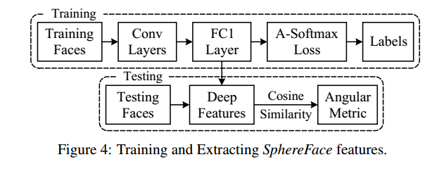
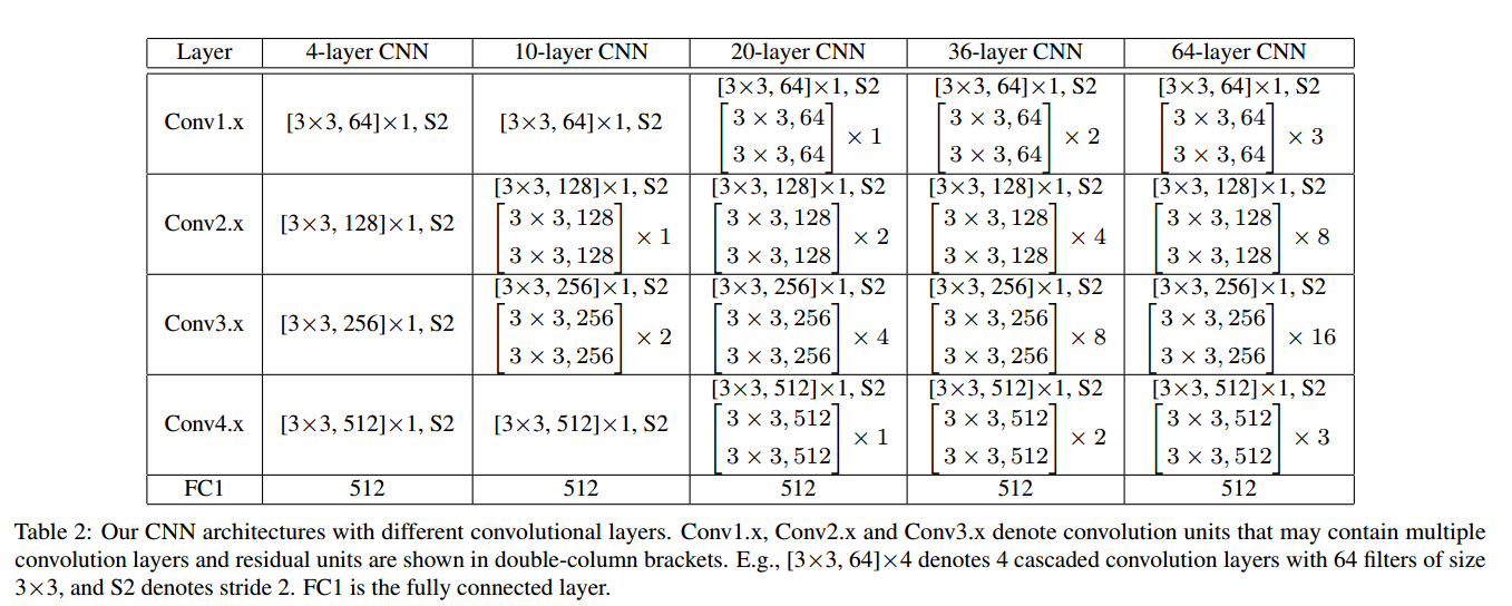
所用的模型如图8所示：

图8

效果如下所示（详细的对比，请看原文）：

图9

A-Softmax在较小的数据集合上有着良好的效果且理论具有不错的可解释性，它的缺点也明显就是计算量相对比较大，也许这就是作者在论文中没有测试大数据集的原因。

与L-Softmax的区别

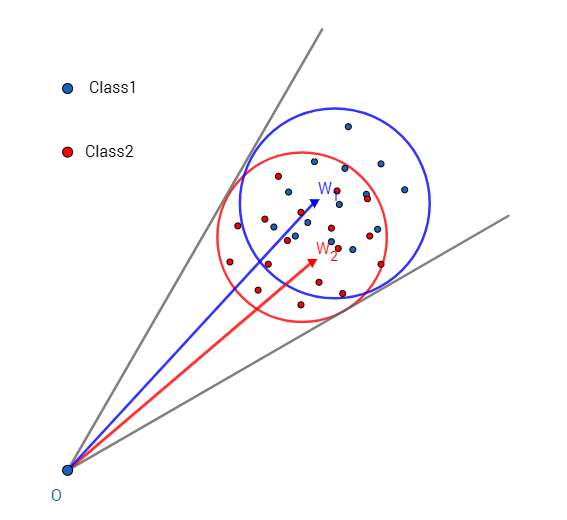
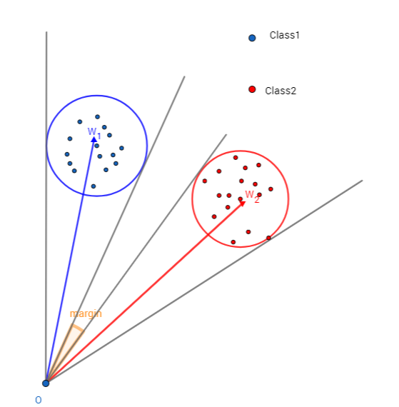
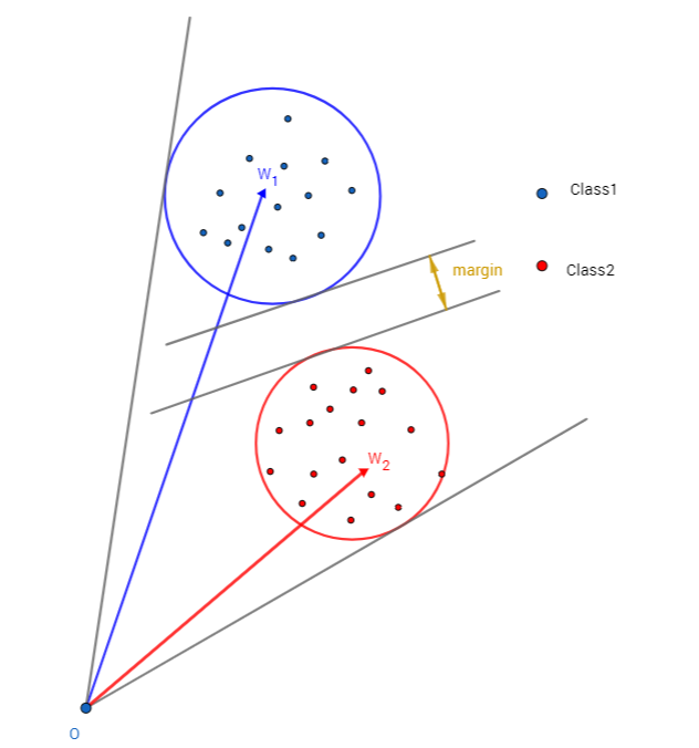
A-Softmax与L-Softmax的最大区别在于A-Softmax的权重归一化了，而L-Softmax则没的。A-Softmax权重的归一化导致特征上的点映射到单位超球面上，而L-Softmax则不没有这个限制，这个特性使得两者在几何的解释上是不一样的。如图10所示，如果在训练时两个类别的特征输入在同一个区域时，如下图10所示。A-Softmax只能从角度上分度这两个类别，也就是说它仅从方向上区分类，分类的结果如图11所示；而L-Softmax，不仅可以从角度上区别两个类，还能从权重的模（长度）上区别这两个类，分类的结果如图12所示。在数据集合大小固定的条件下，L-Softmax能有两个方法分类，训练可能没有使得它在角度与长度方向都分离，导致它的精确可能不如A-Softmax。

图10：类别1与类别2映射到特征空间发生了区域的重叠

图11：A-Softmax分类可能的结果

图12：L-Softmax分类可能的结果

【防止爬虫转载而导致的格式问题——链接】：http://www.cnblogs.com/heguanyou/p/7503025.html