
Tensorflow2.0进阶学习-一些自定义操作 (八)
之前都是用model.fit()来训练模型,有没有一种方法可以像PyTorch那样,我可以掌握每一代的数据呢?有的,也是写for循环的。 Customization basics
张量操作
import tensorflow as tf

print(tf.math.add(1, 2))  # 简单相加
print(tf.math.add([1, 2], [3, 4]))  # 矩阵对应元素相加
print(tf.math.square(5))  # 数值的平方
print(tf.math.reduce_sum([1, 2, 3]))  # 数组的和

# Operator overloading is also supported
print(tf.math.square(2) + tf.math.square(3))  # 简单的加减乘除符号也是可以的
结果,和Numpy的格式也差不多。
tf.Tensor(3, shape=(), dtype=int32)
tf.Tensor([4 6], shape=(2,), dtype=int32)
tf.Tensor(25, shape=(), dtype=int32)
tf.Tensor(6, shape=(), dtype=int32)
tf.Tensor(13, shape=(), dtype=int32)
来看下tf.Tensor 的格式
x = tf.linalg.matmul([[1]], [[2, 3]])  # 相乘
print(x)
print(x.shape)
print(x.dtype)
结果,可以看到里面有三个东西,一个是数值,一个是数据的形状shape,一个是数据类型dtype
tf.Tensor([[2 3]], shape=(1, 2), dtype=int32)
(1, 2)
<dtype: 'int32'>
张量有GPU、TPU的支持,张量也是不可变得,张量和NumPy可以相互转换。
下面代码就是一个相互转换的例子。
import numpy as np

ndarray = np.ones([3, 3])

print("TensorFlow operations convert numpy arrays to Tensors automatically")
tensor = tf.math.multiply(ndarray, 42)
print(tensor)


print("And NumPy operations convert Tensors to NumPy arrays automatically")
print(np.add(tensor, 1))

print("The .numpy() method explicitly converts a Tensor to a numpy array")
print(tensor.numpy())
结果
TensorFlow operations convert numpy arrays to Tensors automatically
tf.Tensor(
[[42. 42. 42.]
 [42. 42. 42.]
 [42. 42. 42.]], shape=(3, 3), dtype=float64)
And NumPy operations convert Tensors to NumPy arrays automatically
[[43. 43. 43.]
 [43. 43. 43.]
 [43. 43. 43.]]
The .numpy() method explicitly converts a Tensor to a numpy array
[[42. 42. 42.]
 [42. 42. 42.]
 [42. 42. 42.]]
在TensorFlow 会自动决定是使用 GPU 还是 CPU 进行操作
x = tf.random.uniform([3, 3])

print("Is there a GPU available: "),
print(tf.config.list_physical_devices("GPU"))

print("Is the Tensor on GPU #0:  "),
print(x.device.endswith('GPU:0'))
结果
Is there a GPU available:
[PhysicalDevice(name='/physical_device:GPU:0', device_type='GPU')]
Is the Tensor on GPU #0:
True
当然也可以自行决定存放数据在CPU或者某个GPU上
import time

def time_matmul(x):
  start = time.time()
  for loop in range(10):
    tf.linalg.matmul(x, x)

  result = time.time()-start

  print("10 loops: {:0.2f}ms".format(1000*result))

# Force execution on CPU
print("On CPU:")
with tf.device("CPU:0"):
  x = tf.random.uniform([1000, 1000])
  assert x.device.endswith("CPU:0")
  time_matmul(x)

# Force execution on GPU #0 if available
if tf.config.list_physical_devices("GPU"):
  print("On GPU:")
  with tf.device("GPU:0"): # Or GPU:1 for the 2nd GPU, GPU:2 for the 3rd etc.
    x = tf.random.uniform([1000, 1000])
    assert x.device.endswith("GPU:0")
    time_matmul(x)
结果
On CPU:
10 loops: 46.04ms
On GPU:
2022-05-02 17:01:30.919764: I tensorflow/stream_executor/cuda/cuda_blas.cc:1786] TensorFloat-32 will be used for the matrix multiplication. This will only be logged once.
10 loops: 680.97ms
数据集也可以自定义
可以使用函数tf.data.Dataset.from_tensors , tf.data.Dataset.from_tensor_slices,tf.data.TextLineDataset 和tf.data.TFRecordDataset等等系列,去定义数据集。
例子
ds_tensors = tf.data.Dataset.from_tensor_slices([1, 2, 3, 4, 5, 6])

# Create a CSV file
import tempfile
_, filename = tempfile.mkstemp()

with open(filename, 'w') as f:
  f.write("""Line 1
Line 2
Line 3
  """)

ds_file = tf.data.TextLineDataset(filename)
也可以有一些转换方法
tf.data.Dataset.map,tf.data.Dataset.batch 和 tf.data.Dataset.shuffle等来对数据集进行设置定制。
ds_tensors = ds_tensors.map(tf.math.square).shuffle(2).batch(2)

ds_file = ds_file.batch(2)
tf.data.Dataset 支持循环迭代查看信息,也就是for循环打印。
print('Elements of ds_tensors:')
for x in ds_tensors:
  print(x)

print('\nElements in ds_file:')
for x in ds_file:
  print(x)
打印出来的信息
Elements of ds_tensors:
tf.Tensor([1 4], shape=(2,), dtype=int32)
tf.Tensor([ 9 16], shape=(2,), dtype=int32)
tf.Tensor([36 25], shape=(2,), dtype=int32)
Elements in ds_file:
tf.Tensor([b'Line 1' b'Line 2'], shape=(2,), dtype=string)
tf.Tensor([b'Line 3' b'  '], shape=(2,), dtype=string)
网络层操作
import tensorflow as tf

print(tf.config.list_physical_devices('GPU'))
# [PhysicalDevice(name='/physical_device:GPU:0', device_type='GPU')]
先看下Tensorflow为我们写好的网络层。
定义一层全连接层网络,第一个参数是数据出来的最后维度,第二个参数是输入数据的维度,可以略,因为网络自己就可以推断出来。所有的网络层都可以在这找到
# In the tf.keras.layers package, layers are objects. To construct a layer,
# simply construct the object. Most layers take as a first argument the number
# of output dimensions / channels.
layer = tf.keras.layers.Dense(100)
# The number of input dimensions is often unnecessary, as it can be inferred
# the first time the layer is used, but it can be provided if you want to
# specify it manually, which is useful in some complex models.
layer = tf.keras.layers.Dense(10, input_shape=(None, 5))
做一个数据,塞进去看看什么结果
# To use a layer, simply call it.
layer(tf.zeros([10, 5]))
数据的形状变了,变成[10, 10],最后维度和全连接层的第一个参数就一致了。
<tf.Tensor: shape=(10, 10), dtype=float32, numpy=
array([[0., 0., 0., 0., 0., 0., 0., 0., 0., 0.],
       [0., 0., 0., 0., 0., 0., 0., 0., 0., 0.],
       [0., 0., 0., 0., 0., 0., 0., 0., 0., 0.],
       [0., 0., 0., 0., 0., 0., 0., 0., 0., 0.],
       [0., 0., 0., 0., 0., 0., 0., 0., 0., 0.],
       [0., 0., 0., 0., 0., 0., 0., 0., 0., 0.],
       [0., 0., 0., 0., 0., 0., 0., 0., 0., 0.],
       [0., 0., 0., 0., 0., 0., 0., 0., 0., 0.],
       [0., 0., 0., 0., 0., 0., 0., 0., 0., 0.],
       [0., 0., 0., 0., 0., 0., 0., 0., 0., 0.]], dtype=float32)>
当然也可以看看网络层里的参数是什么
# Layers have many useful methods. For example, you can inspect all variables
# in a layer using `layer.variables` and trainable variables using
# `layer.trainable_variables`. In this case a fully-connected layer
# will have variables for weights and biases.
print(layer.variables)
结果
[<tf.Variable 'dense_1/kernel:0' shape=(5, 10) dtype=float32, numpy=
 array([[ 0.32855886,  0.04384887,  0.02992123,  0.12625396, -0.19404814,
          0.1421498 ,  0.06281334,  0.3417716 , -0.14824864,  0.57778424],
        [-0.5431969 , -0.20277733, -0.559383  ,  0.1770094 ,  0.53273505,
          0.08685184, -0.51780874,  0.42599815,  0.09632635,  0.01097667],
        [ 0.02511215, -0.2831529 , -0.46403354,  0.0624103 ,  0.2874459 ,
          0.43649322, -0.05893129, -0.58793306,  0.3282966 , -0.21102232],
        [ 0.4881131 ,  0.02165043, -0.61608166, -0.45918524, -0.58056116,
          0.11609119, -0.1180836 , -0.43469104,  0.29003525,  0.06869155],
        [ 0.12409163, -0.11788273,  0.1904366 , -0.37554052, -0.32007664,
         -0.18741989,  0.24887705, -0.2900794 ,  0.19865537,  0.00872332]],
       dtype=float32)>,
 <tf.Variable 'dense_1/bias:0' shape=(10,) dtype=float32, numpy=array([0., 0., 0., 0., 0., 0., 0., 0., 0., 0.], dtype=float32)>]
可以看见里面的核参数以及偏置量,就是一个矩阵,[10, 5] 与 [5 ,10]的矩阵相乘就出来[10, 10]。
如果自己想要从头开始,怎么做呢?那就一步步实现好了。
三个方法实现下:
__init__方法可以做一切无关输入张量的操作,我理解就是初始化。build方法就是知道了输入的张量维度了,就接着把剩下的初始化都弄好了,比如设定下进来数据需要多少个参数做运算什么的。call方法就是执行操作了,也就是前向运算。
也可以在__init__ 方法将build里的初始化一并做了,但是这个需要我们传入输入张量的维度。
class MyDenseLayer(tf.keras.layers.Layer):
  def __init__(self, num_outputs):
    super(MyDenseLayer, self).__init__()
    self.num_outputs = num_outputs

  def build(self, input_shape):
    self.kernel = self.add_weight("kernel",
                                  shape=[int(input_shape[-1]),
                                         self.num_outputs])

  def call(self, inputs):
    return tf.matmul(inputs, self.kernel)
# 这里只执行 __init__ 方法
layer = MyDenseLayer(10)
# 这里依次执行 build 和 call
_ = layer(tf.zeros([10, 5])) # Calling the layer `.builds` it.
print([var.name for var in layer.trainable_variables])
# 输出和定义模型名字有观,大写的有下滑线。
# ['my_dense_layer/kernel:0']
除了可以自定义层,还可以对简单的层进行组合,直接看例子
class ResnetIdentityBlock(tf.keras.Model):
  def __init__(self, kernel_size, filters):
    super(ResnetIdentityBlock, self).__init__(name='')
    filters1, filters2, filters3 = filters

    self.conv2a = tf.keras.layers.Conv2D(filters1, (1, 1))
    self.bn2a = tf.keras.layers.BatchNormalization()

    self.conv2b = tf.keras.layers.Conv2D(filters2, kernel_size, padding='same')
    self.bn2b = tf.keras.layers.BatchNormalization()

    self.conv2c = tf.keras.layers.Conv2D(filters3, (1, 1))
    self.bn2c = tf.keras.layers.BatchNormalization()

  def call(self, input_tensor, training=False):
    x = self.conv2a(input_tensor)
    x = self.bn2a(x, training=training)
    x = tf.nn.relu(x)

    x = self.conv2b(x)
    x = self.bn2b(x, training=training)
    x = tf.nn.relu(x)

    x = self.conv2c(x)
    x = self.bn2c(x, training=training)

    x += input_tensor
    return tf.nn.relu(x)


block = ResnetIdentityBlock(1, [1, 2, 3])
# 运行下
_ = block(tf.zeros([1, 2, 3, 3]))
打印里面网络层信息
[<keras.layers.convolutional.Conv2D at 0x226cce82fa0>,
 <keras.layers.normalization.batch_normalization.BatchNormalization at 0x226cce9ed90>,
 <keras.layers.convolutional.Conv2D at 0x226d330a4f0>,
 <keras.layers.normalization.batch_normalization.BatchNormalization at 0x226d32cb070>,
 <keras.layers.convolutional.Conv2D at 0x226d32cbd90>,
 <keras.layers.normalization.batch_normalization.BatchNormalization at 0x226d32cbe20>]
这个块里有多少种参数可训练,18种,包含核向量、偏置量等等。
len(block.variables) # 18
整体结构
block.summary()
结果清清楚楚。
Model: ""
_________________________________________________________________
 Layer (type)                Output Shape              Param #
=================================================================
 conv2d (Conv2D)             multiple                  4

 batch_normalization (BatchN  multiple                 4
 ormalization)

 conv2d_1 (Conv2D)           multiple                  4

 batch_normalization_1 (Batc  multiple                 8
 hNormalization)

 conv2d_2 (Conv2D)           multiple                  9

 batch_normalization_2 (Batc  multiple                 12
 hNormalization)

=================================================================
Total params: 41
Trainable params: 29
Non-trainable params: 12
_________________________________________________________________
如果是顺序执行的化,还可以用tf.keras.Sequential来组合简单层。
my_seq = tf.keras.Sequential([tf.keras.layers.Conv2D(1, (1, 1),
                                                    input_shape=(
                                                        None, None, 3)),
                             tf.keras.layers.BatchNormalization(),
                             tf.keras.layers.Conv2D(2, 1,
                                                    padding='same'),
                             tf.keras.layers.BatchNormalization(),
                             tf.keras.layers.Conv2D(3, (1, 1)),
                             tf.keras.layers.BatchNormalization()])
my_seq(tf.zeros([1, 2, 3, 3]))
这个和上面那个是一样的,结果
<tf.Tensor: shape=(1, 2, 3, 3), dtype=float32, numpy=
array([[[[0., 0., 0.],
         [0., 0., 0.],
         [0., 0., 0.]],
        [[0., 0., 0.],
         [0., 0., 0.],
         [0., 0., 0.]]]], dtype=float32)>
看下结构,看结构的时候必须执行my_seq(tf.zeros([1, 2, 3, 3])),主要是为了执行build函数。
my_seq.summary()
结果为
Model: "sequential_1"
_________________________________________________________________
 Layer (type)                Output Shape              Param #
=================================================================
 conv2d_6 (Conv2D)           (None, None, None, 1)     4

 batch_normalization_6 (Batc  (None, None, None, 1)    4
 hNormalization)

 conv2d_7 (Conv2D)           (None, None, None, 2)     4

 batch_normalization_7 (Batc  (None, None, None, 2)    8
 hNormalization)

 conv2d_8 (Conv2D)           (None, None, None, 3)     9

 batch_normalization_8 (Batc  (None, None, None, 3)    12
 hNormalization)

=================================================================
Total params: 41
Trainable params: 29
Non-trainable params: 12
_________________________________________________________________
自定义训练
来体会下不同于.fit训练的感觉。
- 数据集的导入与解析
- 选择模型类型
- 对模型进行训练
- 评估模型效果
- 使用训练过的模型进行预测
引包
import os
import matplotlib.pyplot as plt

import tensorflow as tf

print("TensorFlow version: {}".format(tf.__version__))
print("Eager execution: {}".format(tf.executing_eagerly()))
数据准备
鸢尾花分类问题,下载数据
train_dataset_url = "https://storage.googleapis.com/download.tensorflow.org/data/iris_training.csv"

train_dataset_fp = tf.keras.utils.get_file(fname=os.path.basename(train_dataset_url),
                                           origin=train_dataset_url)

print("Local copy of the dataset file: {}".format(train_dataset_fp))
纯文本数据,CSV格式的表格数据,解析数据,前四个数字是鸢尾花的四个参数,最后一个代表了它的标签。
# column order in CSV file
column_names = ['sepal_length', 'sepal_width', 'petal_length', 'petal_width', 'species']

feature_names = column_names[:-1]
label_name = column_names[-1]

print("Features: {}".format(feature_names))
print("Label: {}".format(label_name))
- 0 : 山鸢尾
- 1 : 变色鸢尾
- 2 : 维吉尼亚鸢尾
class_names = ['山鸢尾', '变色鸢尾', '维吉尼亚鸢尾']
放入tf.data.Dataset里
CSV格式的数据直接用 make_csv_dataset函数来加载
batch_size = 32

train_dataset = tf.data.experimental.make_csv_dataset(
    train_dataset_fp,
    batch_size,
    column_names=column_names,
    label_name=label_name,
    num_epochs=1)

features, labels = next(iter(train_dataset))

print(features)
结果
OrderedDict([
('sepal_length', <tf.Tensor: shape=(32,), dtype=float32, numpy=
array([6.7, 6.3, 5.1, 5.7, 4.9, 6.8, 6.7, 4.8, 6.1, 7.3, 7.4, 5.3, 5.8,
       4.8, 6.2, 4.7, 5. , 6.3, 6.2, 5.5, 5.7, 7.6, 4.8, 6.6, 5. , 6.1,
       7.7, 5.1, 5.2, 5.7, 6.4, 5.9], dtype=float32)>),
('sepal_width', <tf.Tensor: shape=(32,), dtype=float32, numpy=
array([3. , 2.5, 3.5, 4.4, 2.4, 3.2, 3.1, 3. , 2.6, 2.9, 2.8, 3.7, 2.6,
       3.4, 2.2, 3.2, 3.5, 2.3, 2.8, 3.5, 2.8, 3. , 3. , 3. , 2. , 2.9,
       3. , 3.8, 3.4, 3.8, 2.8, 3.2], dtype=float32)>),
('petal_length', <tf.Tensor: shape=(32,), dtype=float32, numpy=
array([5. , 5. , 1.4, 1.5, 3.3, 5.9, 4.4, 1.4, 5.6, 6.3, 6.1, 1.5, 4. ,
       1.6, 4.5, 1.3, 1.6, 4.4, 4.8, 1.3, 4.1, 6.6, 1.4, 4.4, 3.5, 4.7,
       6.1, 1.9, 1.4, 1.7, 5.6, 4.8], dtype=float32)>),
('petal_width', <tf.Tensor: shape=(32,), dtype=float32, numpy=
array([1.7, 1.9, 0.3, 0.4, 1. , 2.3, 1.4, 0.1, 1.4, 1.8, 1.9, 0.2, 1.2,
       0.2, 1.5, 0.2, 0.6, 1.3, 1.8, 0.2, 1.3, 2.1, 0.3, 1.4, 1. , 1.4,
       2.3, 0.4, 0.2, 0.3, 2.1, 1.8], dtype=float32)>)])
用图来展示看看
plt.scatter(features['petal_length'],
            features['sepal_length'],
            c=labels,
            cmap='viridis')

plt.xlabel("Petal length")
plt.ylabel("Sepal length")
plt.show()

CSV出来的数据是字典型的,还是希望弄成单个Tensor。
此函数使用 tf.stack 方法,该方法从张量列表中获取值,并创建指定维度的组合张量
做了一个映射,用的时候调用就可以了。
def pack_features_vector(features, labels):
  """Pack the features into a single array."""
  features = tf.stack(list(features.values()), axis=1)
  return features, labels
train_dataset = train_dataset.map(pack_features_vector)

features, labels = next(iter(train_dataset))

print(features[:5])
结果
tf.Tensor(
[[5.4 3.7 1.5 0.2]
 [5.  3.3 1.4 0.2]
 [5.4 3.9 1.7 0.4]
 [6.4 3.1 5.5 1.8]
 [6.7 3.1 5.6 2.4]], shape=(5, 4), dtype=float32)
模型准备
model = tf.keras.Sequential([
  tf.keras.layers.Dense(10, activation=tf.nn.relu, input_shape=(4,)),  # input shape required
  tf.keras.layers.Dense(10, activation=tf.nn.relu),
  tf.keras.layers.Dense(3)
])

predictions = model(features)
print(predictions[:5])

print("Prediction: {}".format(tf.argmax(predictions, axis=1)))
print("    Labels: {}".format(labels))
结果
tf.Tensor(
[[-1.5555569  1.3319032 -0.5449946]
 [-4.7065334  1.8886805 -3.1353095]
 [-4.378022   1.8282304 -2.8600035]
 [-4.568859   1.8847792 -3.0071104]
 [-3.593163   1.4276582 -2.4097426]], shape=(5, 3), dtype=float32)
Prediction: [1 1 1 1 1 1 1 1 1 1 1 1 1 1 1 1 1 1 1 1 1 1 1 1 1 1 1 1 1 1 1 1]
    Labels: [0 2 2 2 1 2 2 1 1 0 1 1 0 0 2 1 0 1 2 0 2 0 0 1 0 2 2 2 2 0 1 2]
跑起来
先定义一个损失函数,这里采用tf.keras.losses.SparseCategoricalCrossentropy函数。
loss_object = tf.keras.losses.SparseCategoricalCrossentropy(from_logits=True)

def loss(model, x, y, training):
  # training=training is needed only if there are layers with different
  # behavior during training versus inference (e.g. Dropout).
  y_ = model(x, training=training)

  return loss_object(y_true=y, y_pred=y_)


l = loss(model, features, labels, training=False)
print("Loss test: {}".format(l))
使用 tf.GradientTape 的前后关系来计算梯度以优化你的模型
def grad(model, inputs, targets):
  with tf.GradientTape() as tape:
    loss_value = loss(model, inputs, targets, training=True)
  return loss_value, tape.gradient(loss_value, model.trainable_variables)
优化器,利用随机梯度下降,反向传播一次。
optimizer = tf.keras.optimizers.SGD(learning_rate=0.01)

loss_value, grads = grad(model, features, labels)

print("Step: {}, Initial Loss: {}".format(optimizer.iterations.numpy(),
                                          loss_value.numpy()))

optimizer.apply_gradients(zip(grads, model.trainable_variables))

print("Step: {},         Loss: {}".format(optimizer.iterations.numpy(),
                                          loss(model, features, labels, training=True).numpy()))
结果
Step: 0, Initial Loss: 1.3080095052719116
Step: 1,         Loss: 1.2500560283660889
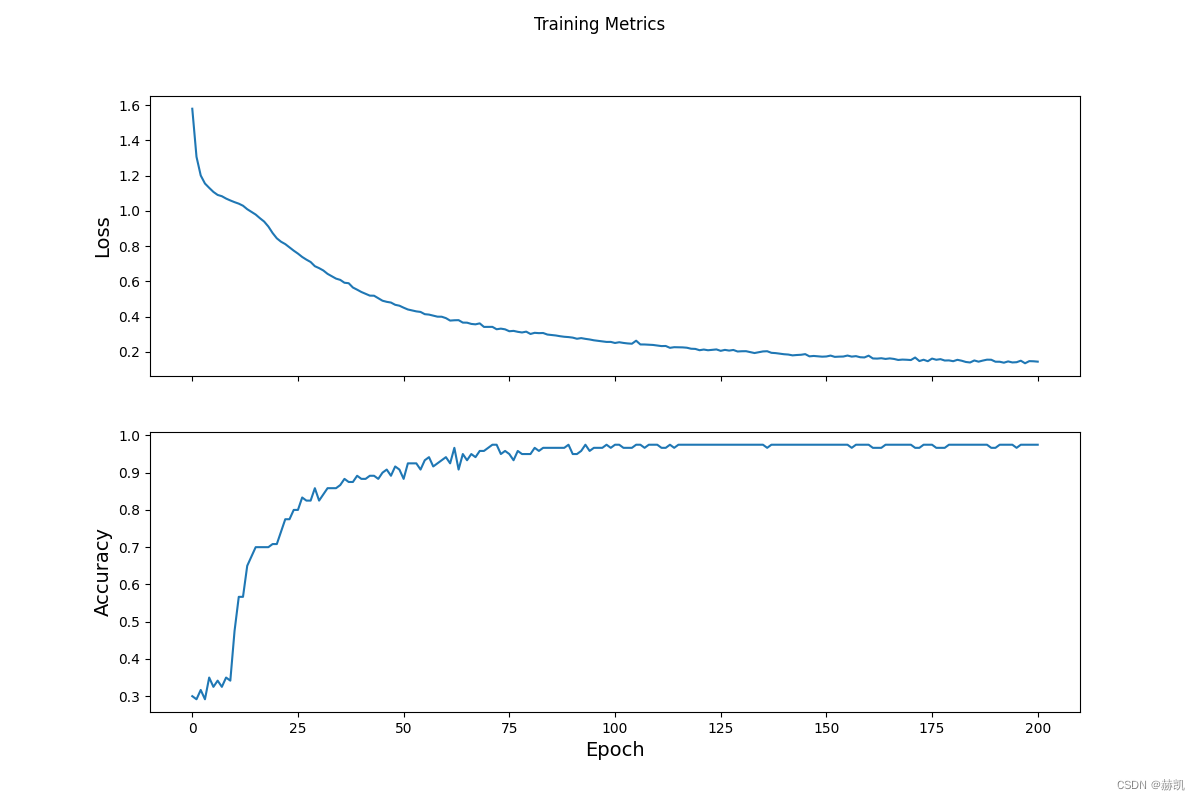
终于可以循环了
- 迭代每个周期。通过一次数据集即为一个周期。
- 在一个周期中,遍历训练 Dataset 中的每个样本,并获取样本的特征(x)和标签(y)。
- 根据样本的特征进行预测,并比较预测结果和标签。衡量预测结果的不准确性,并使用所得的值计算模型的损失和梯度。
- 使用 optimizer更新模型的变量。
- 跟踪一些统计信息以进行可视化。
- 对每个周期重复执行以上步骤。
## Note: Rerunning this cell uses the same model variables

# Keep results for plotting
train_loss_results = []
train_accuracy_results = []

num_epochs = 201

for epoch in range(num_epochs):
  epoch_loss_avg = tf.keras.metrics.Mean()
  epoch_accuracy = tf.keras.metrics.SparseCategoricalAccuracy()

  # Training loop - using batches of 32
  for x, y in train_dataset:
    # Optimize the model
    loss_value, grads = grad(model, x, y)
    optimizer.apply_gradients(zip(grads, model.trainable_variables))

    # Track progress
    epoch_loss_avg.update_state(loss_value)  # Add current batch loss
    # Compare predicted label to actual label
    # training=True is needed only if there are layers with different
    # behavior during training versus inference (e.g. Dropout).
    epoch_accuracy.update_state(y, model(x, training=True))

  # End epoch
  train_loss_results.append(epoch_loss_avg.result())
  train_accuracy_results.append(epoch_accuracy.result())

  if epoch % 50 == 0:
    print("Epoch {:03d}: Loss: {:.3f}, Accuracy: {:.3%}".format(epoch,
                                                                epoch_loss_avg.result(),
                                                                epoch_accuracy.result()))
结果
Epoch 000: Loss: 1.567, Accuracy: 24.167%
Epoch 050: Loss: 0.414, Accuracy: 90.000%
Epoch 100: Loss: 0.261, Accuracy: 96.667%
Epoch 150: Loss: 0.174, Accuracy: 97.500%
Epoch 200: Loss: 0.142, Accuracy: 97.500%
fig, axes = plt.subplots(2, sharex=True, figsize=(12, 8))
fig.suptitle('Training Metrics')

axes[0].set_ylabel("Loss", fontsize=14)
axes[0].plot(train_loss_results)

axes[1].set_ylabel("Accuracy", fontsize=14)
axes[1].set_xlabel("Epoch", fontsize=14)
axes[1].plot(train_accuracy_results)
plt.show()
评估
test_url = "https://storage.googleapis.com/download.tensorflow.org/data/iris_test.csv"

test_fp = tf.keras.utils.get_file(fname=os.path.basename(test_url),
                                  origin=test_url)
# 和训练数据集一样的做法
test_dataset = tf.data.experimental.make_csv_dataset(
    test_fp,
    batch_size,
    column_names=column_names,
    label_name='species',
    num_epochs=1,
    shuffle=False)

test_dataset = test_dataset.map(pack_features_vector)
跑的时候需要model(x, training=False)这样子
test_accuracy = tf.keras.metrics.Accuracy()

for (x, y) in test_dataset:
  # training=False is needed only if there are layers with different
  # behavior during training versus inference (e.g. Dropout).
  logits = model(x, training=False)
  prediction = tf.argmax(logits, axis=1, output_type=tf.int32)
  test_accuracy(prediction, y)

print("Test set accuracy: {:.3%}".format(test_accuracy.result()))
# Test set accuracy: 93.333%
预测,当然可以用前面的保存、加载模型
predict_dataset = tf.convert_to_tensor([
    [5.1, 3.3, 1.7, 0.5,],
    [5.9, 3.0, 4.2, 1.5,],
    [6.9, 3.1, 5.4, 2.1]
])

# training=False is needed only if there are layers with different
# behavior during training versus inference (e.g. Dropout).
predictions = model(predict_dataset, training=False)

for i, logits in enumerate(predictions):
  class_idx = tf.argmax(logits).numpy()
  p = tf.nn.softmax(logits)[class_idx]
  name = class_names[class_idx]
  print("Example {} prediction: {} ({:4.1f}%)".format(i, name, 100*p))
结果
Example 0 prediction: 山鸢尾 (95.7%)
Example 1 prediction: 变色鸢尾 (80.3%)
Example 2 prediction: 维吉尼亚鸢尾 (80.2%)
本文来自博客园,作者:赫凯,转载请注明原文链接:https://www.cnblogs.com/heKaiii/p/17137413.html

 浙公网安备 33010602011771号