
YOLO系列,【YOLOV5-5.x 源码解读】loss.py
转载:https://blog.csdn.net/qq_38253797/article/details/119444854 建议前往原文阅读,非常精彩,这里仅当学习记录
目录
前言
0、导入需要的包
1、smooth_BCE
2、BCEBlurWithLogitsLoss
3、FocalLoss
4、QFocalLoss
5、ComputeLoss类
5.1、__init__函数
5.2、build_targets
5.3、__call__函数
总结
Reference
前言
源码: YOLOv5源码.
导航: 【YOLOV5-5.x 源码讲解】整体项目文件导航.
注释版全部项目文件已上传至GitHub: yolov5-5.x-annotations.
这个文件是yolov5的损失函数部分。代码量不多,只有300多行,但却是整个项目最难,最精华的部分。在看这个文件之前建议大家仔细看下下面两篇关于BCE交叉熵损失函数的内容: 【PyTorch 理论】交叉熵损失函数的理解 和 【PyTorch】两种常用的交叉熵损失函数BCELoss和BCEWithLogitsLoss 。另外,这个文件涉及到了损失函数的计算、正负样本取样、平滑标签增强、Focalloss、QFocalloss等操作,都是比较常用的trick,一样都要弄懂!
0、导入需要的包
import torch
import torch.nn as nn

from utils.metrics import bbox_iou
from utils.torch_utils import is_parallel
1、smooth_BCE
这个函数是一个标签平滑的策略(trick),是一种在 分类/检测 问题中,防止过拟合的方法。如果要详细理解这个策略的原理,可以看看我的另一篇博文: 【trick 1】Label Smoothing(标签平滑)—— 分类问题中错误标注的一种解决方法.
smooth_BCE函数代码。
def smooth_BCE(eps=0.1):
    """用在ComputeLoss类中
    标签平滑操作  [1, 0]  =>  [0.95, 0.05]
    https://github.com/ultralytics/yolov3/issues/238#issuecomment-598028441
    :params eps: 平滑参数
    :return positive, negative label smoothing BCE targets  两个值分别代表正样本和负样本的标签取值
            原先的正样本=1 负样本=0 改为 正样本=1.0 - 0.5 * eps  负样本=0.5 * eps
    """
    return 1.0 - 0.5 * eps, 0.5 * eps
通常会用在分类损失当中,如下ComputeLoss类的__init__函数定义:

ComputeLoss类的__call__函数调用:

2、BCEBlurWithLogitsLoss
这个函数是BCE函数的一个替代,是yolov5作者的一个实验性的函数,可以自己试试效果。
class BCEBlurWithLogitsLoss(nn.Module):
    """用在ComputeLoss类的__init__函数中
    BCEwithLogitLoss() with reduced missing label effects.
    https://github.com/ultralytics/yolov5/issues/1030
    The idea was to reduce the effects of false positive (missing labels) 就是检测成正样本了 但是检测错了
    """
    def __init__(self, alpha=0.05):
        super(BCEBlurWithLogitsLoss, self).__init__()
        self.loss_fcn = nn.BCEWithLogitsLoss(reduction='none')  # must be nn.BCEWithLogitsLoss()
        self.alpha = alpha

    def forward(self, pred, true):
        loss = self.loss_fcn(pred, true)
        pred = torch.sigmoid(pred)  # prob from logits
        # dx = [-1, 1]  当pred=1 true=0时(网络预测说这里有个obj但是gt说这里没有), dx=1 => alpha_factor=0 => loss=0
        # 这种就是检测成正样本了但是检测错了(false positive)或者missing label的情况 这种情况不应该过多的惩罚->loss=0
        dx = pred - true  # reduce only missing label effects
        # 如果采样绝对值的话 会减轻pred和gt差异过大而造成的影响
        # dx = (pred - true).abs()  # reduce missing label and false label effects
        alpha_factor = 1 - torch.exp((dx - 1) / (self.alpha + 1e-4))
        loss *= alpha_factor
        return loss.mean()
使用起来直接在ComputeLoss类的__init__函数中替代传统的BCE函数即可:

3、FocalLoss
FocalLoss损失函数来自 Kaiming He在2017年发表的一篇论文:Focal Loss for Dense Object Detection. 这篇论文设计的主要思路: 希望那些hard examples对损失的贡献变大,使网络更倾向于从这些样本上学习。防止由于easy examples过多,主导整个损失函数。
优点:
- 解决了one-stage object detection中图片中正负样本(前景和背景)不均衡的问题;
- 降低简单样本的权重,使损失函数更关注困难样本;
函数公式:

更多细节请看我的另一篇博客: 【trick 4】Focal Loss —— 解决one-stage目标检测中正负样本不均衡的问题
FocalLoss函数代码:
class FocalLoss(nn.Module):
    """用在代替原本的BCEcls(分类损失)和BCEobj(置信度损失)
    Wraps focal loss around existing loss_fcn(), i.e. criteria = FocalLoss(nn.BCEWithLogitsLoss(), gamma=1.5)
    论文: https://arxiv.org/abs/1708.02002
    https://blog.csdn.net/qq_38253797/article/details/116292496
    TF implementation https://github.com/tensorflow/addons/blob/v0.7.1/tensorflow_addons/losses/focal_loss.py
    """
    def __init__(self, loss_fcn, gamma=1.5, alpha=0.25):
        super(FocalLoss, self).__init__()
        self.loss_fcn = loss_fcn  # must be nn.BCEWithLogitsLoss()=Sigmoid+BCELoss  定义为多分类交叉熵损失函数
        self.gamma = gamma   # 参数gamma  用于削弱简单样本对loss的贡献程度
        self.alpha = alpha   # 参数alpha  用于平衡正负样本个数不均衡的问题
        # self.reduction: 控制FocalLoss损失输出模式 sum/mean/none   默认是Mean
        self.reduction = loss_fcn.reduction
        # focalloss中的BCE函数的reduction='None'  BCE不使用Sum或者Mean
        self.loss_fcn.reduction = 'none'  # 需要将Focal loss应用于每一个样本之中

    def forward(self, pred, true):
        loss = self.loss_fcn(pred, true)   # 正常BCE的loss:   loss = -log(p_t)
        # p_t = torch.exp(-loss)
        # loss *= self.alpha * (1.000001 - p_t) ** self.gamma  # non-zero power for gradient stability

        pred_prob = torch.sigmoid(pred)  # prob from logits
        # true=1 p_t=pred_prob    true=0 p_t=1-pred_prob
        p_t = true * pred_prob + (1 - true) * (1 - pred_prob)   # p_t
        # true=1 alpha_factor=self.alpha    true=0 alpha_factor=1-self.alpha
        alpha_factor = true * self.alpha + (1 - true) * (1 - self.alpha)  # alpha_t
        modulating_factor = (1.0 - p_t) ** self.gamma  # 这里代表Focal loss中的指数项
        # 返回最终的loss=BCE * 两个参数  (看看公式就行了 和公式一模一样)
        loss *= alpha_factor * modulating_factor

        # 最后选择focalloss返回的类型 默认是mean
        if self.reduction == 'mean':
            return loss.mean()
        elif self.reduction == 'sum':
            return loss.sum()
        else:  # 'none'
            return loss
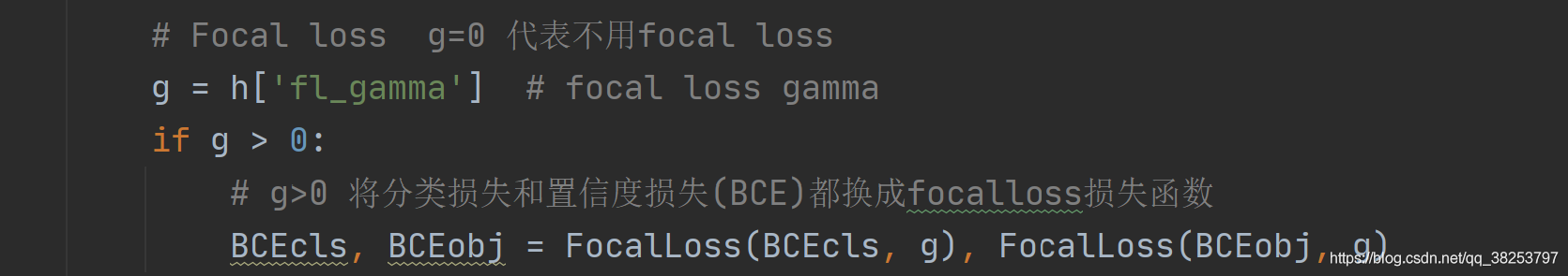
这个函数用在代替原本的BCEcls和BCEobj:
4、QFocalLoss
QFocalLoss损失函数来自20年的一篇文章: Generalized Focal Loss: Learning Qualified and Distributed Bounding Boxes for Dense Object Detection.
这篇文章我暂时还没有看完,因为涉及太多的anchor free的内容,后面学完anchor free的一些经典论文再回来重写。
如果对这篇论文感兴趣可以看看大神博客: 大白话 Generalized Focal Loss.
公式:
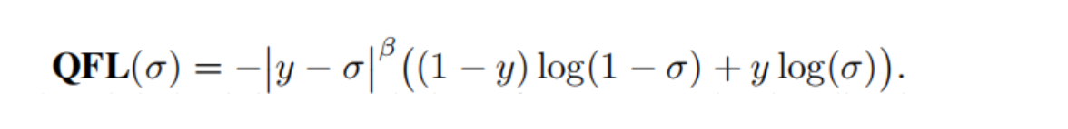
QFocalLoss函数代码:
class QFocalLoss(nn.Module):
    """用来代替FocalLoss
    QFocalLoss 来自General Focal Loss论文: https://arxiv.org/abs/2006.04388
    Wraps Quality focal loss around existing loss_fcn(), i.e. criteria = FocalLoss(nn.BCEWithLogitsLoss(), gamma=1.5)
    """
    def __init__(self, loss_fcn, gamma=1.5, alpha=0.25):
        super(QFocalLoss, self).__init__()
        self.loss_fcn = loss_fcn  # must be nn.BCEWithLogitsLoss()
        self.gamma = gamma
        self.alpha = alpha
        self.reduction = loss_fcn.reduction
        self.loss_fcn.reduction = 'none'  # required to apply FL to each element

    def forward(self, pred, true):
        loss = self.loss_fcn(pred, true)

        pred_prob = torch.sigmoid(pred)  # prob from logits
        alpha_factor = true * self.alpha + (1 - true) * (1 - self.alpha)
        # 和FocalLoss相比只变了这里
        modulating_factor = torch.abs(true - pred_prob) ** self.gamma
        loss *= alpha_factor * modulating_factor

        if self.reduction == 'mean':
            return loss.mean()
        elif self.reduction == 'sum':
            return loss.sum()
        else:  # 'none'
            return loss
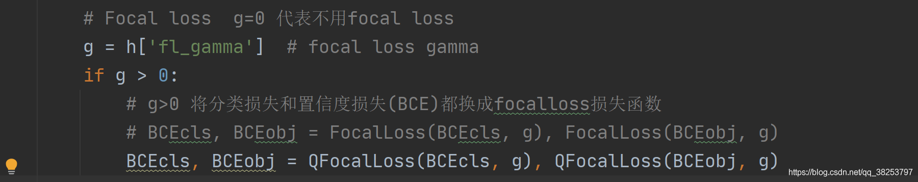
用法就是直接在ComputeLoss时代替FocalLoss即可:
5、ComputeLoss类
5.1、__init__函数
      def __init__(self, model, autobalance=False):
        super(ComputeLoss, self).__init__()
        self.sort_obj_iou = False  # 后面筛选置信度损失正样本的时候是否先对iou排序

        device = next(model.parameters()).device  # get model device
        h = model.hyp  # hyperparameters

        # Define criteria 定义分类损失和置信度损失
        # BCEcls = BCEBlurWithLogitsLoss()
        # BCEobj = BCEBlurWithLogitsLoss()
        # h['cls_pw']=1  BCEWithLogitsLoss默认的正样本权重也是1
        BCEcls = nn.BCEWithLogitsLoss(pos_weight=torch.tensor([h['cls_pw']], device=device))
        BCEobj = nn.BCEWithLogitsLoss(pos_weight=torch.tensor([h['obj_pw']], device=device))

        # 标签平滑  eps=0代表不做标签平滑-> cp=1 cn=0  eps!=0代表做标签平滑 cp代表positive的标签值 cn代表negative的标签值
        self.cp, self.cn = smooth_BCE(eps=h.get('label_smoothing', 0.0))  # positive, negative BCE targets

        # Focal loss  g=0 代表不用focal loss
        g = h['fl_gamma']  # focal loss gamma
        if g > 0:
            # g>0 将分类损失和置信度损失(BCE)都换成focalloss损失函数
            BCEcls, BCEobj = FocalLoss(BCEcls, g), FocalLoss(BCEobj, g)
            # BCEcls, BCEobj = QFocalLoss(BCEcls, g), QFocalLoss(BCEobj, g)

        # det: 返回的是模型的检测头 Detector 3个 分别对应产生三个输出feature map
        det = model.module.model[-1] if is_parallel(model) else model.model[-1]  # Detect() module

        # balance用来设置三个feature map对应输出的置信度损失系数(平衡三个feature map的置信度损失)
        # 从左到右分别对应大feature map(检测小目标)到小feature map(检测大目标)
        # 思路:  It seems that larger output layers may overfit earlier, so those numbers may need a bit of adjustment
        #       一般来说,检测小物体的难度大一点,所以会增加大特征图的损失系数,让模型更加侧重小物体的检测
        # 如果det.nl=3就返回[4.0, 1.0, 0.4]否则返回[4.0, 1.0, 0.25, 0.06, .02]
        # self.balance = {3: [4.0, 1.0, 0.4], 4: [4.0, 1.0, 0.25, 0.06], 5: [4.0, 1.0, 0.25, 0.06, .02]}[det.nl]
        self.balance = {3: [4.0, 1.0, 0.4]}.get(det.nl, [4.0, 1.0, 0.25, 0.06, .02])  # P3-P7

        # 三个预测头的下采样率det.stride: [8, 16, 32]  .index(16): 求出下采样率stride=16的索引
        # 这个参数会用来自动计算更新3个feature map的置信度损失系数self.balance
        self.ssi = list(det.stride).index(16) if autobalance else 0  # stride 16 index

        # self.BCEcls: 类别损失函数   self.BCEobj: 置信度损失函数   self.hyp: 超参数
        # self.gr: 计算真实框的置信度标准的iou ratio    self.autobalance: 是否自动更新各feature map的置信度损失平衡系数  默认False
        self.BCEcls, self.BCEobj, self.gr, self.hyp, self.autobalance = BCEcls, BCEobj, model.gr, h, autobalance

        # na: number of anchors  每个grid_cell的anchor数量 = 3
        # nc: number of classes  数据集的总类别 = 80
        # nl: number of detection layers   Detect的个数 = 3
        # anchors: [3, 3, 2]  3个feature map 每个feature map上有3个anchor(w,h) 这里的anchor尺寸是相对feature map的
        for k in 'na', 'nc', 'nl', 'anchors':
            # setattr: 给对象self的属性k赋值为getattr(det, k)
            # getattr: 返回det对象的k属性
            # 所以这句话的意思: 讲det的k属性赋值给self.k属性 其中k in 'na', 'nc', 'nl', 'anchors'
            setattr(self, k, getattr(det, k))
5.2、build_targets
这个函数是用来为所有GT筛选相应的anchor正样本。筛选条件是比较GT和anchor的宽比和高比,大于一定的阈值就是负样本,反之正样本。筛选到的正样本信息(image_index, anchor_index, gridy, gridx),传入__call__函数,通过这个信息去筛选pred每个grid预测得到的信息,保留对应grid_cell上的正样本。通过build_targets筛选的GT中的正样本和pred筛选出的对应位置的预测样本进行计算损失。
补充理解:这个函数的目的是为了每个gt匹配相应的高质量anchor正样本参与损失计算,j = torch.max(r, 1. / r).max(2)[0] < self.hyp[‘anchor_t’]这步的比较是为了将gt分配到不同层上去检测(和你说的差不多),后面的步骤是为了将确定在这层检测的gt中心坐标,进而确定这个gt在这层哪个grid cell进行检测。做到这一步也就做到了为每个gt匹配anchor正样本的目的。
    def build_targets(self, p, targets):
        """所有GT筛选相应的anchor正样本
        Build targets for compute_loss()
        :params p: p[i]的作用只是得到每个feature map的shape
                   预测框 由模型构建中的三个检测头Detector返回的三个yolo层的输出
                   tensor格式 list列表 存放三个tensor 对应的是三个yolo层的输出
                   如: [4, 3, 112, 112, 85]、[4, 3, 56, 56, 85]、[4, 3, 28, 28, 85]
                   [bs, anchor_num, grid_h, grid_w, xywh+class+classes]
                   可以看出来这里的预测值p是三个yolo层每个grid_cell(每个grid_cell有三个预测值)的预测值,后面肯定要进行正样本筛选
        :params targets: 数据增强后的真实框 [63, 6] [num_target,  image_index+class+xywh] xywh为归一化后的框
        :return tcls: 表示这个target所属的class index
                tbox: xywh 其中xy为这个target对当前grid_cell左上角的偏移量
                indices: b: 表示这个target属于的image index
                         a: 表示这个target使用的anchor index
                        gj: 经过筛选后确定某个target在某个网格中进行预测(计算损失)  gj表示这个网格的左上角y坐标
                        gi: 表示这个网格的左上角x坐标
                anch: 表示这个target所使用anchor的尺度(相对于这个feature map)  注意可能一个target会使用大小不同anchor进行计算
        """
        na, nt = self.na, targets.shape[0]  # number of anchors 3, targets 63
        tcls, tbox, indices, anch = [], [], [], []   # 初始化tcls tbox indices anch

        # gain是为了后面将targets=[na,nt,7]中的归一化了的xywh映射到相对feature map尺度上
        # 7: image_index+class+xywh+anchor_index
        gain = torch.ones(7, device=targets.device)

        # 需要在3个anchor上都进行训练 所以将标签赋值na=3个  ai代表3个anchor上在所有的target对应的anchor索引 就是用来标记下当前这个target属于哪个anchor
        # [1, 3] -> [3, 1] -> [3, 63]=[na, nt]   三行  第一行63个0  第二行63个1  第三行63个2
        ai = torch.arange(na, device=targets.device).float().view(na, 1).repeat(1, nt)  # same as .repeat_interleave(nt)

        # [63, 6] [3, 63] -> [3, 63, 6] [3, 63, 1] -> [3, 63, 7]  7: [image_index+class+xywh+anchor_index]
        # 对每一个feature map: 这一步是将target复制三份 对应一个feature map的三个anchor
        # 先假设所有的target都由这层的三个anchor进行检测(复制三份)  再进行筛选  并将ai加进去标记当前是哪个anchor的target
        targets = torch.cat((targets.repeat(na, 1, 1), ai[:, :, None]), 2)  # append anchor indices

        # 这两个变量是用来扩展正样本的 因为预测框预测到target有可能不止当前的格子预测到了
        # 可能周围的格子也预测到了高质量的样本 我们也要把这部分的预测信息加入正样本中
        g = 0.5  # bias  中心偏移  用来衡量target中心点离哪个格子更近
        # 以自身 + 周围左上右下4个网格 = 5个网格  用来计算offsets
        off = torch.tensor([[0, 0],
                            [1, 0], [0, 1], [-1, 0], [0, -1],  # j,k,l,m
                            # [1, 1], [1, -1], [-1, 1], [-1, -1],  # jk,jm,lk,lm
                            ], device=targets.device).float() * g  # offsets

        # 遍历三个feature 筛选gt的anchor正样本
        for i in range(self.nl):  # self.nl: number of detection layers   Detect的个数 = 3
            # anchors: 当前feature map对应的三个anchor尺寸(相对feature map)  [3, 2]
            anchors = self.anchors[i]

            # gain: 保存每个输出feature map的宽高 -> gain[2:6]=gain[whwh]
            # [1, 1, 1, 1, 1, 1, 1] -> [1, 1, 112, 112, 112,112, 1]=image_index+class+xywh+anchor_index
            gain[2:6] = torch.tensor(p[i].shape)[[3, 2, 3, 2]]  # xyxy gain

            # t = [3, 63, 7]  将target中的xywh的归一化尺度放缩到相对当前feature map的坐标尺度
            #     [3, 63, image_index+class+xywh+anchor_index]
            t = targets * gain

            if nt:  # 开始匹配  Matches
                # t=[na, nt, 7]   t[:, :, 4:6]=[na, nt, 2]=[3, 63, 2]
                # anchors[:, None]=[na, 1, 2]
                # r=[na, nt, 2]=[3, 63, 2]
                # 所有的gt与当前层的三个anchor的宽高比(w/w  h/h)
                r = t[:, :, 4:6] / anchors[:, None]  # wh ratio (w/w  h/h)

                # 筛选条件  GT与anchor的宽比或高比超过一定的阈值 就当作负样本
                # torch.max(r, 1. / r)=[3, 63, 2] 筛选出宽比w1/w2 w2/w1 高比h1/h2 h2/h1中最大的那个
                # .max(2)返回宽比 高比两者中较大的一个值和它的索引  [0]返回较大的一个值
                # j: [3, 63]  False: 当前anchor是当前gt的负样本  True: 当前anchor是当前gt的正样本
                j = torch.max(r, 1. / r).max(2)[0] < self.hyp['anchor_t']  # compare
                # yolov3 v4的筛选方法: wh_iou  GT与anchor的wh_iou超过一定的阈值就是正样本
                # j = wh_iou(anchors, t[:, 4:6]) > model.hyp['iou_t']  # iou(3,n)=wh_iou(anchors(3,2), gwh(n,2))

                # 根据筛选条件j, 过滤负样本, 得到所有gt的anchor正样本(batch_size张图片)
                # 知道当前gt的坐标 属于哪张图片 正样本对应的idx 也就得到了当前gt的正样本anchor
                # t: [3, 63, 7] -> [126, 7]  [num_Positive_sample, image_index+class+xywh+anchor_index]
                t = t[j]  # filter

                # Offsets 筛选当前格子周围格子 找到2个离target中心最近的两个格子  可能周围的格子也预测到了高质量的样本 我们也要把这部分的预测信息加入正样本中
                # 除了target所在的当前格子外, 还有2个格子对目标进行检测(计算损失) 也就是说一个目标需要3个格子去预测(计算损失)
                # 首先当前格子是其中1个 再从当前格子的上下左右四个格子中选择2个 用这三个格子去预测这个目标(计算损失)
                # feature map上的原点在左上角 向右为x轴正坐标 向下为y轴正坐标
                gxy = t[:, 2:4]  # grid xy 取target中心的坐标xy(相对feature map左上角的坐标)
                gxi = gain[[2, 3]] - gxy  # inverse  得到target中心点相对于右下角的坐标  gain[[2, 3]]为当前feature map的wh
                # 筛选中心坐标 距离当前grid_cell的左、上方偏移小于g=0.5 且 中心坐标必须大于1(坐标不能在边上 此时就没有4个格子了)
                # j: [126] bool 如果是True表示当前target中心点所在的格子的左边格子也对该target进行回归(后续进行计算损失)
                # k: [126] bool 如果是True表示当前target中心点所在的格子的上边格子也对该target进行回归(后续进行计算损失)
                j, k = ((gxy % 1. < g) & (gxy > 1.)).T
                # 筛选中心坐标 距离当前grid_cell的右、下方偏移小于g=0.5 且 中心坐标必须大于1(坐标不能在边上 此时就没有4个格子了)
                # l: [126] bool 如果是True表示当前target中心点所在的格子的右边格子也对该target进行回归(后续进行计算损失)
                # m: [126] bool 如果是True表示当前target中心点所在的格子的下边格子也对该target进行回归(后续进行计算损失)
                l, m = ((gxi % 1. < g) & (gxi > 1.)).T
                # j: [5, 126]  torch.ones_like(j): 当前格子, 不需要筛选全是True  j, k, l, m: 左上右下格子的筛选结果
                j = torch.stack((torch.ones_like(j), j, k, l, m))
                # 得到筛选后所有格子的正样本 格子数<=3*126 都不在边上等号成立
                # t: [126, 7] -> 复制5份target[5, 126, 7]  分别对应当前格子和左上右下格子5个格子
                # j: [5, 126] + t: [5, 126, 7] => t: [378, 7] 理论上是小于等于3倍的126 当且仅当没有边界的格子等号成立
                t = t.repeat((5, 1, 1))[j]
                # torch.zeros_like(gxy)[None]: [1, 126, 2]   off[:, None]: [5, 1, 2]  => [5, 126, 2]
                # j筛选后: [378, 2]  得到所有筛选后的网格的中心相对于这个要预测的真实框所在网格边界(左右上下边框)的偏移量
                offsets = (torch.zeros_like(gxy)[None] + off[:, None])[j]
            else:
                t = targets[0]
                offsets = 0

            # Define
            b, c = t[:, :2].long().T  # image_index, class
            gxy = t[:, 2:4]  # target的xy
            gwh = t[:, 4:6]  # target的wh
            gij = (gxy - offsets).long()   # 预测真实框的网格所在的左上角坐标(有左上右下的网格)
            gi, gj = gij.T  # grid xy indices

            # Append
            a = t[:, 6].long()  # anchor index
            # b: image index  a: anchor index  gj: 网格的左上角y坐标  gi: 网格的左上角x坐标
            indices.append((b, a, gj.clamp_(0, gain[3] - 1), gi.clamp_(0, gain[2] - 1)))
            # tbix: xywh 其中xy为这个target对当前grid_cell左上角的偏移量
            tbox.append(torch.cat((gxy - gij, gwh), 1))  # box
            anch.append(anchors[a])  # 对应的所有anchors
            tcls.append(c)  # class

        return tcls, tbox, indices, anch
5.3、__call__函数
这个函数相当于forward函数,在这个函数中进行损失函数的前向传播。
        def __call__(self, p, targets):  # predictions, targets, model
        """
        :params p:  预测框 由模型构建中的三个检测头Detector返回的三个yolo层的输出
                    tensor格式 list列表 存放三个tensor 对应的是三个yolo层的输出
                    如: [4, 3, 112, 112, 85]、[4, 3, 56, 56, 85]、[4, 3, 28, 28, 85]
                    [bs, anchor_num, grid_h, grid_w, xywh+class+classes]
                    可以看出来这里的预测值p是三个yolo层每个grid_cell(每个grid_cell有三个预测值)的预测值,后面肯定要进行正样本筛选
        :params targets: 数据增强后的真实框 [63, 6] [num_object,  batch_index+class+xywh]
        :params loss * bs: 整个batch的总损失  进行反向传播
        :params torch.cat((lbox, lobj, lcls, loss)).detach(): 回归损失、置信度损失、分类损失和总损失 这个参数只用来可视化参数或保存信息
        """
        device = targets.device  # 确定运行的设备

        # 初始化lcls, lbox, lobj三种损失值  tensor([0.])
        lcls, lbox, lobj = torch.zeros(1, device=device), torch.zeros(1, device=device), torch.zeros(1, device=device)

        # 每一个都是append的 有feature map个 每个都是当前这个feature map中3个anchor筛选出的所有的target(3个grid_cell进行预测)
        # tcls: 表示这个target所属的class index
        # tbox: xywh 其中xy为这个target对当前grid_cell左上角的偏移量
        # indices: b: 表示这个target属于的image index
        #          a: 表示这个target使用的anchor index
        #          gj: 经过筛选后确定某个target在某个网格中进行预测(计算损失)  gj表示这个网格的左上角y坐标
        #          gi: 表示这个网格的左上角x坐标
        # anch: 表示这个target所使用anchor的尺度(相对于这个feature map)  注意可能一个target会使用大小不同anchor进行计算
        tcls, tbox, indices, anchors = self.build_targets(p, targets)  # targets

        # 依次遍历三个feature map的预测输出pi,这里有三个yolo层的输出,就会遍历三次
        for i, pi in enumerate(p):  # layer index, layer predictions,每一个predictions包括[bs, anchor_num,grid_h,grid_w,xywh+class+classes]
            b, a, gj, gi = indices[i]  # image_index, anchor_index, gridy, gridx

            tobj = torch.zeros_like(pi[..., 0], device=device)  # 初始化target置信度(先全是负样本 后面再筛选正样本赋值)

            n = b.shape[0]  # number of targets
            if n:
                # 精确得到第b张图片的第a个feature map的grid_cell(gi, gj)对应的预测值
                # 用这个预测值与我们筛选的这个grid_cell的真实框进行预测(计算损失)
                ps = pi[b, a, gj, gi]  # prediction subset corresponding to targets,得到的是xywh+class+classes

                # Regression loss  只计算所有正样本的回归损失
                # 新的公式:  pxy = [-0.5 + cx, 1.5 + cx]    pwh = [0, 4pw]   这个区域内都是正样本
                # Get more positive samples, accelerate convergence and be more stable
                pxy = ps[:, :2].sigmoid() * 2. - 0.5  # 一个归一化操作 和论文里不同
                # https://github.com/ultralytics/yolov3/issues/168
                pwh = (ps[:, 2:4].sigmoid() * 2) ** 2 * anchors[i]  # 和论文里不同 这里是作者自己提出的公式
                pbox = torch.cat((pxy, pwh), 1)  # predicted box
                # 这里的tbox[i]中的xy是这个target对当前grid_cell左上角的偏移量[0,1]  而pbox.T是一个归一化的值
                # 就是要用这种方式训练 传回loss 修改梯度 让pbox越来越接近tbox(偏移量)
                iou = bbox_iou(pbox.T, tbox[i], x1y1x2y2=False, CIoU=True)  # iou(prediction, target)
                lbox += (1.0 - iou).mean()  # iou loss

                # Objectness loss stpe1
                # iou.detach()  不会更新iou梯度  iou并不是反向传播的参数 所以不需要反向传播梯度信息
                score_iou = iou.detach().clamp(0).type(tobj.dtype)  # .clamp(0)必须大于等于0
                # 这里对iou进行排序在做一个优化:当一个正样本出现多个GT的情况也就是同一个grid中有两个gt(密集型且形状差不多物体)
                # There maybe several GTs match the same anchor when calculate ComputeLoss in the scene with dense targets
                if self.sort_obj_iou:
                    # https://github.com/ultralytics/yolov5/issues/3605
                    # There maybe several GTs match the same anchor when calculate ComputeLoss in the scene with dense targets
                    sort_id = torch.argsort(score_iou)  # score从小到大排序 拿到对应index
                    # 排序之后 如果同一个grid出现两个gt 那么我们经过排序之后每个grid中的score_iou都能保证是最大的
                    # (小的会被覆盖 因为同一个grid坐标肯定相同)那么从时间顺序的话, 最后1个总是和最大的IOU去计算LOSS, 梯度传播
                    b, a, gj, gi, score_iou = b[sort_id], a[sort_id], gj[sort_id], gi[sort_id], score_iou[sort_id]
                # 预测信息有置信度 但是真实框信息是没有置信度的 所以需要我们人为的给一个标准置信度
                # self.gr是iou ratio [0, 1]  self.gr越大置信度越接近iou  self.gr越小置信度越接近1(人为加大训练难度)
                tobj[b, a, gj, gi] = (1.0 - self.gr) + self.gr * score_iou  # iou ratio
                # tobj[b, a, gj, gi] = 1  # 如果发现预测的score不高 数据集目标太小太拥挤 困难样本过多 可以试试这个

                # Classification loss  只计算所有正样本的分类损失
                if self.nc > 1:  # cls loss (only if multiple classes)
                    # targets 原本负样本是0  这里使用smooth label 就是cn
                    t = torch.full_like(ps[:, 5:], self.cn, device=device)
                    t[range(n), tcls[i]] = self.cp  # 筛选到的正样本对应位置值是cp
                    lcls += self.BCEcls(ps[:, 5:], t)  # BCE

                # Append targets to text file
                # with open('targets.txt', 'a') as file:
                #     [file.write('%11.5g ' * 4 % tuple(x) + '\n') for x in torch.cat((txy[i], twh[i]), 1)]

            # Objectness loss stpe2 置信度损失是用所有样本(正样本 + 负样本)一起计算损失的
            obji = self.BCEobj(pi[..., 4], tobj)
            # 每个feature map的置信度损失权重不同  要乘以相应的权重系数self.balance[i]
            # 一般来说,检测小物体的难度大一点,所以会增加大特征图的损失系数,让模型更加侧重小物体的检测
            lobj += obji * self.balance[i]  # obj loss

            if self.autobalance:
                # 自动更新各个feature map的置信度损失系数
                self.balance[i] = self.balance[i] * 0.9999 + 0.0001 / obji.detach().item()

        if self.autobalance:
            self.balance = [x / self.balance[self.ssi] for x in self.balance]

        # 根据超参中的损失权重参数 对各个损失进行平衡  防止总损失被某个损失所左右
        lbox *= self.hyp['box']
        lobj *= self.hyp['obj']
        lcls *= self.hyp['cls']

        bs = tobj.shape[0]  # batch size

        loss = lbox + lobj + lcls  # 平均每张图片的总损失

        # loss * bs: 整个batch的总损失
        # .detach()  利用损失值进行反向传播 利用梯度信息更新的是损失函数的参数 而对于损失这个值是不需要梯度反向传播的
        return loss * bs, torch.cat((lbox, lobj, lcls, loss)).detach()
rain.py初始化损失函数类

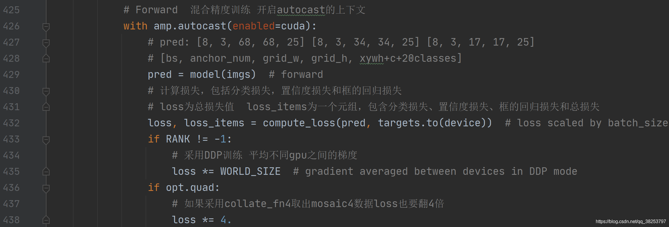
调用执行损失函数,计算损失
总结
这个脚本最最最重要的就是ComputeLoss类了。看了很久,本来打算写细一点的,但是看完代码发现自己把想说的都已经写在代码的注释当中了。代码其实还是挺难的,尤其build_target各种花里胡哨的矩阵操作较多,pytorch不熟的人会看的比较痛苦,但是如果你坚持看下来我的注释再加上自己的debug的话,应该是能读懂的。最后,一定要细读ComputeLoss!!!
另外这个脚本设计到的几个其他的函数可以在这里查看到:【YOLOV5-5.x 源码讲解】整体项目文件导航
Reference
链接1: 博客1.
链接2: 博客2.
链接3: 博客3.
链接4: 博客4.
链接5: 博客5.
————————————————
版权声明:本文为CSDN博主「满船清梦压星河HK」的原创文章,遵循CC 4.0 BY-SA版权协议,转载请附上原文出处链接及本声明。
原文链接:https://blog.csdn.net/qq_38253797/article/details/119444854
posted on 2022-12-20 11:08 Sanny.Liu-CV&&ML 阅读(1147) 评论(0) 收藏 举报


 浙公网安备 33010602011771号