吴恩达深度学习 第二课第二周编程作业_Optimization Methods 优化方法
Optimization Methods 优化方法
参考了 念师 12. 优化算法实战
直到现在,你一直在使用梯度下降来更新参数和最小化代价。在这个笔记本中,你将学习到更先进的优化方法,可以加快学习,甚至可能让你得到一个更好的最终价值的成本函数。有一个好的优化算法,可以是等待几天还是只需几个小时就可以得到一个好的结果。
梯度下降在代价函数J上相当于“下坡”。你可以这样想:

**Figure 1** : **Minimizing the cost is like finding the lowest point in a hilly landscape** 图1 使成本最小化就像在丘陵地带找到最低点
在训练的每一步中,您都要按照一定的方向更新参数,以尝试达到可能的最低点。
符号:一般地, ,对于任何的变量a
首先,运行以下代码导入所需的库。
import numpy as np
import matplotlib.pyplot as plt
import scipy.io
import math
import sklearn
import sklearn.datasets

from opt_utils import load_params_and_grads, initialize_parameters, forward_propagation, backward_propagation
from opt_utils import compute_cost, predict, predict_dec, plot_decision_boundary, load_dataset
from testCases import *

%matplotlib inline
plt.rcParams['figure.figsize'] = (7.0, 4.0) # set default size of plots
plt.rcParams['image.interpolation'] = 'nearest'
plt.rcParams['image.cmap'] = 'gray'
1-Gradient Descent 梯度下降
机器学习中一个简单的优化方法是梯度下降法(GD)。当你对每一步的m个例子进行梯度运算时,它也被称为批量梯度下降。
热身练习:实现梯度下降更新规则。梯度下降规则为,对于l=1,…,l:
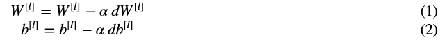
式中,L为层数,a为学习率。所有参数都应该存储在参数字典中。注意,在for循环中迭代器 l 从0开始,而第一个参数是W[1]和b[1]。编码时需要将 l 转换为 l+1。


 1 # GRADED FUNCTION: update_parameters_with_gd
 2
 3 def update_parameters_with_gd(parameters, grads, learning_rate):
 4     """
 5     Update parameters using one step of gradient descent
 6
 7     Arguments:
 8     parameters -- python dictionary containing your parameters to be updated:
 9                     parameters['W' + str(l)] = Wl
10                     parameters['b' + str(l)] = bl
11     grads -- python dictionary containing your gradients to update each parameters:
12                     grads['dW' + str(l)] = dWl
13                     grads['db' + str(l)] = dbl
14     learning_rate -- the learning rate, scalar.
15
16     Returns:
17     parameters -- python dictionary containing your updated parameters
18     """
19
20     L = len(parameters) // 2 # number of layers in the neural networks
21
22     # Update rule for each parameter
23     for l in range(L):
24         ### START CODE HERE ### (approx. 2 lines)
25         parameters["W" + str(l+1)] = parameters["W" + str(l+1)] - learning_rate*grads["dW" + str(l+1)]
26         parameters["b" + str(l+1)] = parameters["b" + str(l+1)] -learning_rate*grads["db" + str(l+1)]
27         ### END CODE HERE ###
28
29     return parameters
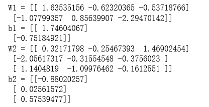
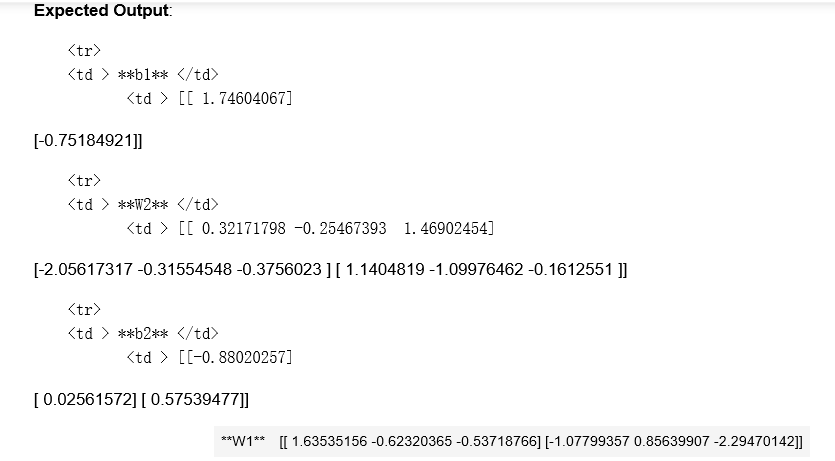
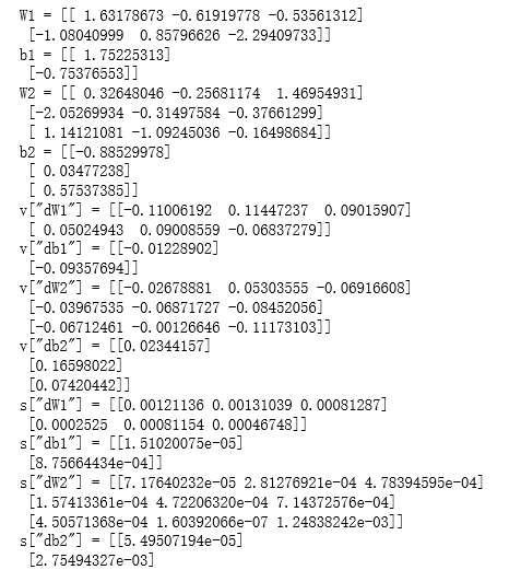
parameters, grads, learning_rate = update_parameters_with_gd_test_case()

parameters = update_parameters_with_gd(parameters, grads, learning_rate)
print("W1 = " + str(parameters["W1"]))
print("b1 = " + str(parameters["b1"]))
print("W2 = " + str(parameters["W2"]))
print("b2 = " + str(parameters["b2"]))
它的一个变体是随机梯度下降(SGD)Stochastic Gradient Descent (SGD),这相当于迷你批梯度下降,其中每个迷你批次只有一个例子。您刚刚实现的更新规则不会更改。改变的是你一次只能在一个训练例子上计算梯度,而不是在整个训练集上。下面的代码例子说明了随机梯度下降和(批处理)梯度下降之间的区别。
(Batch) Gradient Descent:
X = data_input
Y = labels
parameters = initialize_parameters(layers_dims)
for i in range(0, num_iterations):
    # Forward propagation
    a, caches = forward_propagation(X, parameters)
    # Compute cost.
    cost = compute_cost(a, Y)
    # Backward propagation.
    grads = backward_propagation(a, caches, parameters)
    # Update parameters.
    parameters = update_parameters(parameters, grads)
Stochastic Gradient Descent:
X = data_input
Y = labels
parameters = initialize_parameters(layers_dims)
for i in range(0, num_iterations):
    for j in range(0, m):
        # Forward propagation
        a, caches = forward_propagation(X[:,j], parameters)
        # Compute cost
        cost = compute_cost(a, Y[:,j])
        # Backward propagation
        grads = backward_propagation(a, caches, parameters)
        # Update parameters.
        parameters = update_parameters(parameters, grads)
在随机梯度下降中,在更新梯度之前你只使用一个训练例子。当训练集较大时,SGD可以更快(Stochastic 随机的)。但是参数将会朝着最小值“振荡”而不是平滑地收敛。这里有一个例子:

**Figure 1** : **SGD vs GD**
“+”表示成本的最小值。SGD导致许多振荡,以达到收敛。但是,SGD的每一步计算都比GD快得多,因为它只使用一个训练示例(而GD使用整个批处理)。
还要注意,实现SGD总共需要3个for循环:
1.over迭代次数
2.over m个训练例子
3.over 层(更新所有参数,从(W [1],b[1])到(W [L],b [L]))
在实践中,如果不使用整个训练集或只使用一个训练示例来执行每次更新,通常会得到更快的结果。迷你批处理梯度下降对每一步使用中间数量的示例。使用小批量梯度下降,您可以对小批量进行循环,而不是对单个训练示例进行循环。

**Figure 2** : **SGD vs Mini-Batch GD**
“+”表示成本的最小值。在优化算法中使用小批量通常会导致更快的优化。
**你应该记住的**:-梯度下降,小批量梯度下降和随机梯度下降之间的区别是你用来执行一个更新步骤的例子的数量。
-你必须调整一个学习速率超参数。
-与一个良好的小批量大小,通常它优于梯度下降或随机梯度下降(特别是当训练集是大的)。
2 - Mini-Batch Gradient descent
让我们学习如何从训练集(X, Y)构建小批量。
有两个步骤:
•Shuffle:创建一个Shuffle版本的训练集(X, Y),如下图所示。X和Y的每一列代表一个训练示例。注意,随机变换是在X和y之间同步进行的,这样在变换后,X的第i列就是y中第i个标签对应的示例。变换步骤确保示例将被随机分割成不同的小批。

•分区:将打乱的(X, Y)分区到大小为mini_batch_size(此处为64)的迷你批中。注意,训练示例的数量并不总是能被mini_batch_size整除。最后一个迷你批可能更小,但您不需要为此担心。当最后一个迷你批小于完整的mini_batch_size时,它看起来是这样的:

练习:实现random_mini_batches。我们给你编了shuffle部分。为了帮助您完成分区步骤,我们为您提供以下代码,用于选择第1批和第2批的索引:
first_mini_batch_X = shuffled_X[:, 0: mini_batch_size]
second_mini_batch_X = shuffled_X[:, mini_batch_size: 2 * mini_batch_size]
...
注意,最后一个迷你批处理可能小于mini_batch_size=64。让⌊s⌋代表年代四舍五入到最近的整数(这是math.floor (s)在Python中)。如果总数例子不是mini_batch_size = 64的倍数,那么将 满64的例子,例子的数量在最后mini-batch将是
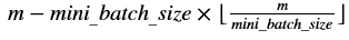 。
。
 1 # GRADED FUNCTION: random_mini_batches
 2
 3 def random_mini_batches(X, Y, mini_batch_size = 64, seed = 0):
 4     """
 5     Creates a list of random minibatches from (X, Y)
 6
 7     Arguments:
 8     X -- input data, of shape (input size, number of examples)
 9     Y -- true "label" vector (1 for blue dot / 0 for red dot), of shape (1, number of examples)
10     mini_batch_size -- size of the mini-batches, integer
11
12     Returns:
13     mini_batches -- list of synchronous (mini_batch_X, mini_batch_Y)
14     """
15
16     np.random.seed(seed)            # To make your "random" minibatches the same as ours
17     m = X.shape[1]                  # number of training examples
18     mini_batches = []
19
20     # Step 1: Shuffle (X, Y)  #第一步:打乱顺序
21     permutation = list(np.random.permutation(m))#它会返回一个长度为m的随机数组,且里面的数是0到m-1 permutation是组合、排列的意思
22     shuffled_X = X[:, permutation] #将每一列的数据按permutation的顺序来重新排列。
23     shuffled_Y = Y[:, permutation].reshape((1,m))
24     """
25     #博博主注:
26     #如果你不好理解的话请看一下下面的伪代码,看看X和Y是如何根据permutation来打乱顺序的。
27     x = np.array([[1,2,3,4,5,6,7,8,9],
28                  [9,8,7,6,5,4,3,2,1]])
29     y = np.array([[1,0,1,0,1,0,1,0,1]])
30
31     random_mini_batches(x,y)
32     permutation= [7, 2, 1, 4, 8, 6, 3, 0, 5]
33     shuffled_X= [[8 3 2 5 9 7 4 1 6]
34                  [2 7 8 5 1 3 6 9 4]]
35     shuffled_Y= [[0 1 0 1 1 1 0 1 0]]
36     """
37
38     # Step 2: Partition (shuffled_X, shuffled_Y). Minus the end case. #第二步,分割  减去最后的情况
39     num_complete_minibatches = math.floor(m/mini_batch_size) # number of mini batches of size mini_batch_size in your partitionning
40     #分区中大小为mini_batch_size的迷你批的数量
41     #把你的训练集分割成多少份,请注意,如果值是99.99,那么返回值是99,剩下的0.99会被舍弃
42     #floor() 返回数字的下舍整数。
43
44     for k in range(0, num_complete_minibatches):
45         ### START CODE HERE ### (approx. 2 lines)
46         mini_batch_X = shuffled_X[: , k * mini_batch_size:(k + 1) * mini_batch_size] #一次64列
47         mini_batch_Y = shuffled_Y[: , k * mini_batch_size:(k + 1) * mini_batch_size]
48         ### END CODE HERE ###
49         mini_batch = (mini_batch_X, mini_batch_Y)
50         mini_batches.append(mini_batch)
51         """
52         #博主注:
53         #如果你不好理解的话请单独执行下面的代码,它可以帮你理解一些。
54         a = np.array([[1,2,3,4,5,6,7,8,9],
55                       [9,8,7,6,5,4,3,2,1],
56                       [1,2,3,4,5,6,7,8,9]])
57         k=1
58         mini_batch_size=3
59         print(a[:,1*3:(1+1)*3]) #从第4列到第6列
60         '''
61         [[4 5 6]
62          [6 5 4]
63          [4 5 6]]
64         '''
65         k=2
66         print(a[:,2*3:(2+1)*3]) #从第7列到第9列
67         '''
68         [[7 8 9]
69          [3 2 1]
70          [7 8 9]]
71         '''
72
73         #看一下每一列的数据你可能就会好理解一些
74
75     """
76     #如果训练集的大小刚好是mini_batch_size的整数倍,那么这里已经处理完了
77     #如果训练集的大小不是mini_batch_size的整数倍,那么最后肯定会剩下一些,我们要把它处理了
78     # Handling the end case (last mini-batch < mini_batch_size) #处理结束情况(最后一个迷你批处理< mini_batch_size)
79     if m % mini_batch_size != 0:
80
81         ### START CODE HERE ### (approx. 2 lines)
82         mini_batch_X = shuffled_X[: , mini_batch_size * num_complete_minibatches : m]#这边冒号后面没东西就是到最后
83         mini_batch_Y = shuffled_X[: , mini_batch_size * num_complete_minibatches : m]
84         ### END CODE HERE ###
85         mini_batch = (mini_batch_X, mini_batch_Y)
86         mini_batches.append(mini_batch)
87
88     return mini_batches
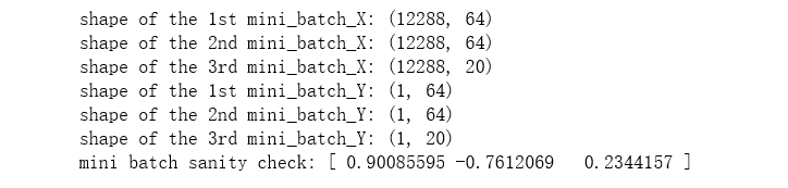
X_assess, Y_assess, mini_batch_size = random_mini_batches_test_case()
mini_batches = random_mini_batches(X_assess, Y_assess, mini_batch_size)

print ("shape of the 1st mini_batch_X: " + str(mini_batches[0][0].shape))
print ("shape of the 2nd mini_batch_X: " + str(mini_batches[1][0].shape))
print ("shape of the 3rd mini_batch_X: " + str(mini_batches[2][0].shape))
print ("shape of the 1st mini_batch_Y: " + str(mini_batches[0][1].shape))
print ("shape of the 2nd mini_batch_Y: " + str(mini_batches[1][1].shape))
print ("shape of the 3rd mini_batch_Y: " + str(mini_batches[2][1].shape))
print ("mini batch sanity check: " + str(mini_batches[0][0][0][0:3]))
**您应该记住的**:——打乱顺序和分区是构建迷你批处理所需的两个步骤——迷你批大小通常选择为2的幂,例如16,32,64,128。
3 - Momentum 动量
因为迷你批处理梯度下降只在看到一个子集的例子后进行参数更新,更新的方向有一些变化,所以迷你批处理梯度下降的路径会朝着收敛方向“振荡”。使用动量可以减少这些振荡。
动量考虑了过去的梯度来平滑更新。我们将把之前梯度的“方向”存储在变量v中。形式上,这将是之前步骤上梯度的指数加权平均值。你也可以把v看作是一个球滚下山的“速度”,根据山坡的坡度/斜坡的方向增加速度(和动量)。
Momentum方法在更新的过程中,考虑了之前时刻的运行方向的影响,最终结合的作用可以克服一些非真实梯度引入的上下抖动现象。

**图3**:红色箭头表示小批量动量梯度下降一步所采取的方向。蓝色的点表示梯度的方向(相对于当前的小批量)在每一步。我们不只是跟随梯度,而是让梯度影响v,然后在v的方向上走一步。
练习:初始化速度。velocity v是一个需要用零数组初始化的python字典。其键值与梯度字典中的键值相同,即:对于l=1,…,l:
v["dW" + str(l+1)] = ... #(numpy array of zeros with the same shape as parameters["W" + str(l+1)])
v["db" + str(l+1)] = ... #(numpy array of zeros with the same shape as parameters["b" + str(l+1)])
注意,迭代器l在for循环中从0开始,而第一个参数是v["dW1"]和v["db1"](上标为"one")。这就是为什么我们要在for循环中将 l 移到 l+1。
# GRADED FUNCTION: initialize_velocity

def initialize_velocity(parameters):
    """
    Initializes the velocity as a python dictionary with:
                - keys: "dW1", "db1", ..., "dWL", "dbL"
                - values: numpy arrays of zeros of the same shape as the corresponding gradients/parameters.
    Arguments:
    parameters -- python dictionary containing your parameters.
                    parameters['W' + str(l)] = Wl
                    parameters['b' + str(l)] = bl

    Returns:
    v -- python dictionary containing the current velocity.
                    v['dW' + str(l)] = velocity of dWl
                    v['db' + str(l)] = velocity of dbl
    """

    L = len(parameters) // 2 # number of layers in the neural networks
    v = {} #v是一个字典

    # Initialize velocity初始化速度
    for l in range(L):
        ### START CODE HERE ### (approx. 2 lines)
        v["dW" + str(l+1)] = np.zeros(parameters['W'+ str(l + 1)].shape)
        v["db" + str(l+1)] = np.zeros(parameters['b'+ str(l + 1)].shape)
        ### END CODE HERE ###

    return v
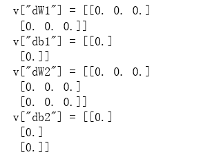
parameters = initialize_velocity_test_case()

v = initialize_velocity(parameters)
print("v[\"dW1\"] = " + str(v["dW1"]))
print("v[\"db1\"] = " + str(v["db1"]))
print("v[\"dW2\"] = " + str(v["dW2"]))
print("v[\"db2\"] = " + str(v["db2"]))
练习:现在,用动量来执行参数更新。动量更新规则为,对于l=1,…,l:
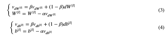
其中,L为层数,β为动量,而α为学习率。所有参数都应该存储在参数字典中。注意,迭代器l在for循环中从0开始,而第一个参数是W[1]和b[1](即上标上的“1”)。所以编码时需要将 l 转换为 l+1。
在momentum中,有一个参数beta。
当beta=0时,此时,momentum相当于没有使用momentum算法的标准梯度下降算法。
当beta越到,说明平滑的作用越明显。通常,在实践中,0.9是比较适当的值。
 1 # GRADED FUNCTION: update_parameters_with_momentum
 2
 3 def update_parameters_with_momentum(parameters, grads, v, beta, learning_rate):
 4     """
 5     Update parameters using Momentum
 6
 7     Arguments:
 8     parameters -- python dictionary containing your parameters:
 9                     parameters['W' + str(l)] = Wl
10                     parameters['b' + str(l)] = bl
11     grads -- python dictionary containing your gradients for each parameters:
12                     grads['dW' + str(l)] = dWl
13                     grads['db' + str(l)] = dbl
14     v -- python dictionary containing the current velocity:
15                     v['dW' + str(l)] = ...
16                     v['db' + str(l)] = ...
17     beta -- the momentum hyperparameter, scalar
18     learning_rate -- the learning rate, scalar
19
20     Returns:
21     parameters -- python dictionary containing your updated parameters
22     v -- python dictionary containing your updated velocities
23     """
24
25     L = len(parameters) // 2 # number of layers in the neural networks
26
27     # Momentum update for each parameter
28     for l in range(L):
29
30         ### START CODE HERE ### (approx. 4 lines)
31         # compute velocities
32         v["dW" + str(l+1)] = beta*v["dW" + str(l+1)] + (1 - beta) * grads['dW' + str(l+1)]
33         v["db" + str(l+1)] = beta*v["db" + str(l+1)] + (1 - beta) * grads['db' + str(l+1)]
34         # update parameters
35         parameters["W" + str(l+1)] = parameters["W" + str(l+1)] - learning_rate * v['dW' + str(l + 1)]
36         parameters["b" + str(l+1)] = parameters["b" + str(l+1)] - learning_rate * v['db' + str(l + 1)]
37         ### END CODE HERE ###
38
39     return parameters, v
parameters, grads, v = update_parameters_with_momentum_test_case()

parameters, v = update_parameters_with_momentum(parameters, grads, v, beta = 0.9, learning_rate = 0.01)
print("W1 = " + str(parameters["W1"]))
print("b1 = " + str(parameters["b1"]))
print("W2 = " + str(parameters["W2"]))
print("b2 = " + str(parameters["b2"]))
print("v[\"dW1\"] = " + str(v["dW1"]))
print("v[\"db1\"] = " + str(v["db1"]))
print("v[\"dW2\"] = " + str(v["dW2"]))
print("v[\"db2\"] = " + str(v["db2"]))
注意:
•速度用零初始化。因此,该算法将需要几次迭代来“提高”速度,并开始采取更大的步骤。
•如果β =0,这就变成了没有动量的标准梯度下降。
你是如何选择β的呢?
•动量值越大,更新就越平滑,因为我们考虑的过去的梯度越多。但如果太大,它也可能平滑的更新太多。
•共值范围从0.8到0.999。如果您不倾向于对其进行调优,那么通常可以使用默认值。
•为你的模型调整最优的调节器可能需要尝试几个值,看看在降低成本函数J的价值方面哪个效果最好。
**你应该记住的**:-动量考虑过去的梯度来平滑梯度下降的步骤。它可以应用于批量梯度下降、小批量梯度下降或随机梯度下降。-你必须调整动量超参数调节器和学习率。
4 - Adam
Adam是训练神经网络最有效的优化算法之一。它结合了RMSProp(讲座中描述的)和Momentum的观点。
Adam是怎么工作的?
1.它计算过去梯度的指数加权平均值,并将其存储在变量v中(偏差校正前)和v校正后
vcorrected(偏差纠正)。
2.它计算过去梯度平方的指数加权平均值,并将其存储在变量s中(偏差校正之前)和s校正
scorrected(偏差纠正)。
3.它结合“1”和“2”的信息,按一定方向更新参数。
更新规则为,对于l=1,…,l:

t 计算Adam所走的步数
•L是层数
•β1和β2是控制两个指数加权平均值的超参数。
•α是学习率
•为了避免被零除,将会出现一个非常小的数字εεε
像往常一样,我们将把所有的参数存储在参数字典中
练习:初始化记录过去信息的Adam变量v,s。
指示:变量v,s是需要用零数组初始化的python字典。其关键字与grads相同,即:l=1时,…,l:
v["dW" + str(l+1)] = ... #(numpy array of zeros with the same shape as parameters["W" + str(l+1)])
v["db" + str(l+1)] = ... #(numpy array of zeros with the same shape as parameters["b" + str(l+1)])
s["dW" + str(l+1)] = ... #(numpy array of zeros with the same shape as parameters["W" + str(l+1)])
s["db" + str(l+1)] = ... #(numpy array of zeros with the same shape as parameters["b" + str(l+1)])
 1 # GRADED FUNCTION: initialize_adam
 2
 3 def initialize_adam(parameters) :
 4     """
 5     Initializes v and s as two python dictionaries with:
 6                 - keys: "dW1", "db1", ..., "dWL", "dbL"
 7                 - values: numpy arrays of zeros of the same shape as the corresponding gradients/parameters.
 8
 9     Arguments:
10     parameters -- python dictionary containing your parameters.
11                     parameters["W" + str(l)] = Wl
12                     parameters["b" + str(l)] = bl
13
14     Returns:
15     v -- python dictionary that will contain the exponentially weighted average of the gradient.
16                     v["dW" + str(l)] = ...
17                     v["db" + str(l)] = ...
18     s -- python dictionary that will contain the exponentially weighted average of the squared gradient.
19                     s["dW" + str(l)] = ...
20                     s["db" + str(l)] = ...
21
22     """
23
24     L = len(parameters) // 2 # number of layers in the neural networks
25     v = {}
26     s = {}
27
28     # Initialize v, s. Input: "parameters". Outputs: "v, s".
29     for l in range(L):
30     ### START CODE HERE ### (approx. 4 lines)
31         v["dW" + str(l+1)] = np.zeros(parameters['W' + str(l + 1)].shape)
32         v["db" + str(l+1)] = np.zeros(parameters['b' + str(l + 1)].shape)
33         s["dW" + str(l+1)] = np.zeros(parameters['W' + str(l + 1)].shape)
34         s["db" + str(l+1)] = np.zeros(parameters['b' + str(l + 1)].shape)
35     ### END CODE HERE ###
36
37     return v, s
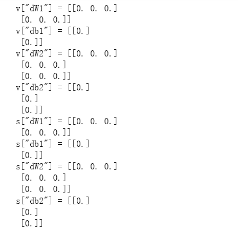
parameters = initialize_adam_test_case()

v, s = initialize_adam(parameters)
print("v[\"dW1\"] = " + str(v["dW1"]))
print("v[\"db1\"] = " + str(v["db1"]))
print("v[\"dW2\"] = " + str(v["dW2"]))
print("v[\"db2\"] = " + str(v["db2"]))
print("s[\"dW1\"] = " + str(s["dW1"]))
print("s[\"db1\"] = " + str(s["db1"]))
print("s[\"dW2\"] = " + str(s["dW2"]))
print("s[\"db2\"] = " + str(s["db2"]))
练习:现在,与Adam一起实现参数更新。回想一下,一般的更新规则是,对于l=1,…,l:

注意,在for循环中迭代器l从0开始,而第一个参数是W [1]和b[1]。编码时需要将l转换为l+1。
 1 # GRADED FUNCTION: update_parameters_with_adam
 2
 3 def update_parameters_with_adam(parameters, grads, v, s, t, learning_rate = 0.01,
 4                                 beta1 = 0.9, beta2 = 0.999,  epsilon = 1e-8):
 5     """
 6     Update parameters using Adam
 7
 8     Arguments:
 9     parameters -- python dictionary containing your parameters:
10                     parameters['W' + str(l)] = Wl
11                     parameters['b' + str(l)] = bl
12     grads -- python dictionary containing your gradients for each parameters:
13                     grads['dW' + str(l)] = dWl
14                     grads['db' + str(l)] = dbl
15     v -- Adam variable, moving average of the first gradient, python dictionary
16     s -- Adam variable, moving average of the squared gradient, python dictionary
17     learning_rate -- the learning rate, scalar.
18     beta1 -- Exponential decay hyperparameter for the first moment estimates
19     beta2 -- Exponential decay hyperparameter for the second moment estimates
20     epsilon -- hyperparameter preventing division by zero in Adam updates
21
22     Returns:
23     parameters -- python dictionary containing your updated parameters
24     v -- Adam variable, moving average of the first gradient, python dictionary
25     s -- Adam variable, moving average of the squared gradient, python dictionary
26     """
27
28     L = len(parameters) // 2                 # number of layers in the neural networks
29     v_corrected = {}                         # Initializing first moment estimate, python dictionary
30     s_corrected = {}                         # Initializing second moment estimate, python dictionary
31
32     # Perform Adam update on all parameters
33     for l in range(L):
34         # Moving average of the gradients. Inputs: "v, grads, beta1". Output: "v".
35         ### START CODE HERE ### (approx. 2 lines)
36         v["dW" + str(l+1)] = beta1*v["dW" + str(l+1)] + (1-beta1)*grads['dW' + str(l+1)]
37         v["db" + str(l+1)] = beta1*v["db" + str(l+1)] + (1-beta1)*grads['db' + str(l+1)]
38         ### END CODE HERE ###
39
40         # Compute bias-corrected first moment estimate. Inputs: "v, beta1, t". Output: "v_corrected".
41         ### START CODE HERE ### (approx. 2 lines)
42         v_corrected["dW" + str(l+1)] =  v["dW" + str(l+1)] / (1-(beta1)**t)
43         v_corrected["db" + str(l+1)] = v["db" + str(l+1)] / (1-(beta1)**t)
44         ### END CODE HERE ###
45
46         # Moving average of the squared gradients. Inputs: "s, grads, beta2". Output: "s".
47         ### START CODE HERE ### (approx. 2 lines)
48         s["dW" + str(l+1)] = beta2*s["dW" + str(l+1)] + (1-beta2)*(grads['dW' + str(l+1)]**2)
49         s["db" + str(l+1)] = beta2*s["db" + str(l+1)] + (1-beta2)*(grads['db' + str(l+1)]**2)
50         ### END CODE HERE ###
51
52         # Compute bias-corrected second raw moment estimate. Inputs: "s, beta2, t". Output: "s_corrected".
53         ### START CODE HERE ### (approx. 2 lines)
54         s_corrected["dW" + str(l+1)] = s["dW" + str(l+1)] / (1-(beta2)**t)
55         s_corrected["db" + str(l+1)] = s["db" + str(l+1)] / (1-(beta2)**t)
56         ### END CODE HERE ###
57
58         # Update parameters. Inputs: "parameters, learning_rate, v_corrected, s_corrected, epsilon". Output: "parameters".
59         ### START CODE HERE ### (approx. 2 lines)
60         parameters["W" + str(l+1)] = parameters['W' + str(l+1)] - learning_rate * (v_corrected["dW" + str(l+1)]/np.sqrt(s_corrected["dW" + str(l+1)] + epsilon))
61         parameters["b" + str(l+1)] = parameters['b' + str(l+1)] - learning_rate * (v_corrected["db" + str(l+1)]/np.sqrt(s_corrected["db" + str(l+1)] + epsilon))
62         ### END CODE HERE ###
63
64     return parameters, v, s
parameters, grads, v, s = update_parameters_with_adam_test_case()
parameters, v, s  = update_parameters_with_adam(parameters, grads, v, s, t = 2)

print("W1 = " + str(parameters["W1"]))
print("b1 = " + str(parameters["b1"]))
print("W2 = " + str(parameters["W2"]))
print("b2 = " + str(parameters["b2"]))
print("v[\"dW1\"] = " + str(v["dW1"]))
print("v[\"db1\"] = " + str(v["db1"]))
print("v[\"dW2\"] = " + str(v["dW2"]))
print("v[\"db2\"] = " + str(v["db2"]))
print("s[\"dW1\"] = " + str(s["dW1"]))
print("s[\"db1\"] = " + str(s["db1"]))
print("s[\"dW2\"] = " + str(s["dW2"]))
print("s[\"db2\"] = " + str(s["db2"]))
您现在有了三种可用的优化算法(mini-batch gradient descent、Momentum和Adam)。让我们用每一个优化器实现一个模型,并观察它们的区别。
5 - Model with different optimization algorithms 模型采用不同的优化算法
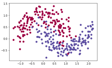
让我们使用下面的“月亮”数据集来测试不同的优化方法。(数据集被命名为“月亮”,因为这两个类的数据看起来都有点像月牙形的月亮。)
train_X, train_Y = load_dataset()
我们已经实现了一个3层的神经网络。你将用:
•Mini-batch梯度下降法:它将调用你的函数:◾update_parameters_with_gd ()
•Mini-batch动量:它将调用你的函数:◾initialize_velocity()和update_parameters_with_momentum ()
•Mini-batch Adam:它将调用你的函数:◾initialize_adam()和update_parameters_with_adam ()
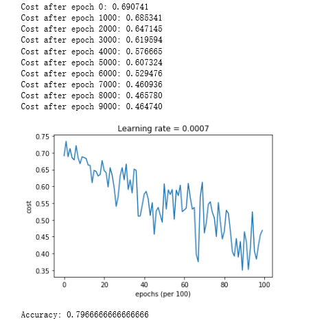
 1 def model(X, Y, layers_dims, optimizer, learning_rate = 0.0007, mini_batch_size = 64, beta = 0.9,
 2           beta1 = 0.9, beta2 = 0.999,  epsilon = 1e-8, num_epochs = 10000, print_cost = True):
 3     """
 4     3-layer neural network model which can be run in different optimizer modes.
 5
 6     Arguments:
 7     X -- input data, of shape (2, number of examples)
 8     Y -- true "label" vector (1 for blue dot / 0 for red dot), of shape (1, number of examples)
 9     layers_dims -- python list, containing the size of each layer
10     learning_rate -- the learning rate, scalar.
11     mini_batch_size -- the size of a mini batch
12     beta -- Momentum hyperparameter
13     beta1 -- Exponential decay hyperparameter for the past gradients estimates
14     beta2 -- Exponential decay hyperparameter for the past squared gradients estimates
15     epsilon -- hyperparameter preventing division by zero in Adam updates
16     num_epochs -- number of epochs
17     print_cost -- True to print the cost every 1000 epochs
18
19     Returns:
20     parameters -- python dictionary containing your updated parameters
21     """
22
23     L = len(layers_dims)             # number of layers in the neural networks
24     costs = []                       # to keep track of the cost
25     t = 0                            # initializing the counter required for Adam update初始化Adam需要的计数
26     seed = 10                        # For grading purposes, so that your "random" minibatches are the same as ours
27
28     # Initialize parameters
29     parameters = initialize_parameters(layers_dims)
30
31     # Initialize the optimizer初始化优化器
32     if optimizer == "gd":
33         pass # no initialization required for gradient descent梯度下降不需要初始化
34     elif optimizer == "momentum":
35         v = initialize_velocity(parameters)
36     elif optimizer == "adam":
37         v, s = initialize_adam(parameters)
38
39     # Optimization loop 优化循环
40     for i in range(num_epochs):
41
42         # Define the random minibatches. We increment the seed to reshuffle differently the dataset after each epoch
43         #定义随机小批。我们增加种子以不同的方式在每个epoch后重新洗牌数据集
44         seed = seed + 1
45         minibatches = random_mini_batches(X, Y, mini_batch_size, seed)
46
47         for minibatch in minibatches:
48
49             # Select a minibatch
50             (minibatch_X, minibatch_Y) = minibatch
51
52             # Forward propagation
53             a3, caches = forward_propagation(minibatch_X, parameters)
54
55             # Compute cost
56             cost = compute_cost(a3, minibatch_Y)
57
58             # Backward propagation
59             grads = backward_propagation(minibatch_X, minibatch_Y, caches)
60
61             # Update parameters更新参数
62             if optimizer == "gd":
63                 parameters = update_parameters_with_gd(parameters, grads, learning_rate)
64             elif optimizer == "momentum":
65                 parameters, v = update_parameters_with_momentum(parameters, grads, v, beta, learning_rate)
66             elif optimizer == "adam":
67                 t = t + 1 # Adam counter
68                 parameters, v, s = update_parameters_with_adam(parameters, grads, v, s,
69                                                                t, learning_rate, beta1, beta2,  epsilon)
70
71         # Print the cost every 1000 epoch
72         if print_cost and i % 1000 == 0:
73             print ("Cost after epoch %i: %f" %(i, cost))
74         if print_cost and i % 100 == 0:
75             costs.append(cost)
76
77     # plot the cost
78     plt.plot(costs)
79     plt.ylabel('cost')
80     plt.xlabel('epochs (per 100)')
81     plt.title("Learning rate = " + str(learning_rate))
82     plt.show()
83
84     return parameters
现在,您将使用3种优化方法中的每一种来运行这个3层神经网络
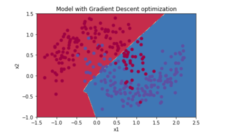
5.1 - Mini-batch Gradient descent 小批量梯度下降
运行以下代码,查看模型如何使用迷你批处理梯度下降。
 1 # train 3-layer model
 2 layers_dims = [train_X.shape[0], 5, 2, 1]
 3 parameters = model(train_X, train_Y, layers_dims, optimizer = "gd")
 4
 5 # Predict
 6 predictions = predict(train_X, train_Y, parameters)
 7
 8 # Plot decision boundary
 9 plt.title("Model with Gradient Descent optimization")
10 axes = plt.gca()
11 axes.set_xlim([-1.5,2.5])
12 axes.set_ylim([-1,1.5])
13 plot_decision_boundary(lambda x: predict_dec(parameters, x.T), train_X, train_Y)

5.2 - Mini-batch gradient descent with momentum
运行下面的代码,查看模型如何使用momentum。因为这个例子相对简单,使用momemtum的好处很小;但对于更复杂的问题,你可能会看到更大的收获。
# train 3-layer model
layers_dims = [train_X.shape[0], 5, 2, 1]
parameters = model(train_X, train_Y, layers_dims, beta = 0.9, optimizer = "momentum")

# Predict
predictions = predict(train_X, train_Y, parameters)

# Plot decision boundary
plt.title("Model with Momentum optimization")
axes = plt.gca()
axes.set_xlim([-1.5,2.5])
axes.set_ylim([-1,1.5])
plot_decision_boundary(lambda x: predict_dec(parameters, x.T), train_X, train_Y)

5.3 - Mini-batch with Adam mode
运行以下代码,查看模型如何处理Adam。
# train 3-layer model
layers_dims = [train_X.shape[0], 5, 2, 1]
parameters = model(train_X, train_Y, layers_dims, optimizer = "adam")

# Predict
predictions = predict(train_X, train_Y, parameters)

# Plot decision boundary
plt.title("Model with Adam optimization")
axes = plt.gca()
axes.set_xlim([-1.5,2.5])
axes.set_ylim([-1,1.5])
plot_decision_boundary(lambda x: predict_dec(parameters, x.T), train_X, train_Y)


5.4 - Summary
不同优化算法的对比结果如下表:
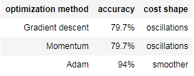
动量通常是有用的,但考虑到学习速度小和数据集简单,它的影响几乎是可以忽略的。而且,你在成本中看到的巨大振荡,来自于优化算法中一些小批量比其他小批量更难处理的事实。
另一方面,Adam明显优于小批量梯度下降和动量。如果您在这个简单的数据集上运行更多的epoch模型,所有三种方法都将得到非常好的结果。但是,Adam的收敛速度更快。
Adam的一些优点包括:
•相对较低的内存需求(尽管高于梯度下降和动量梯度下降)
•通常工作得很好,即使只有很少的超参数调整(除了α)
References:
- Adam paper: https://arxiv.org/pdf/1412.6980.pdf
作者:Agiroy_70
本博客所有文章仅用于学习、研究和交流目的,欢迎非商业性质转载。
博主的文章主要是记录一些学习笔记、作业等。文章来源也已表明,由于博主的水平不高,不足和错误之处在所难免,希望大家能够批评指出。
博主是利用读书、参考、引用、抄袭、复制和粘贴等多种方式打造成自己的文章,请原谅博主成为一个无耻的文档搬运工!

 浙公网安备 33010602011771号