Note2-基于MNE实现脑电源定位的论文级别可视化
摘要
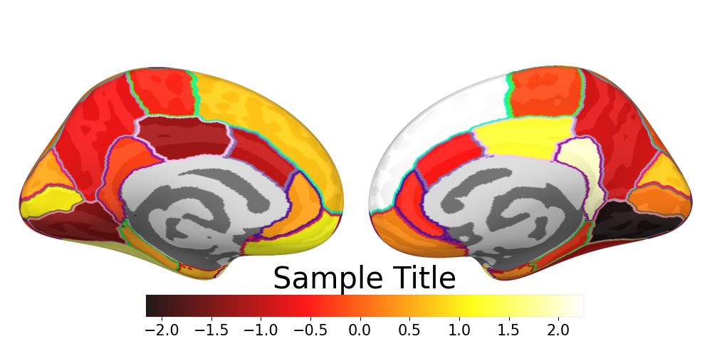
好的可视化能够清楚直观地展示实验结果。脑电(EEG)目前常见的研究往往基于头皮地形图进行可视化,解释层次仅止步于额叶/颞叶/顶叶/枕叶,对于大脑机理的解释粒度较为粗糙。通过源定位+可视化,能够让研究结果更为细腻,展示不同脑区的神经活动表现。本文基于MNE框架实现论文级直接可用的可视化,示例如下图所示。脑区划分方式/colorbar颜色均可自行调整。

环境准备与脑电源定位提取
可 点击链接参考上一篇博客。
可视化代码实现与解析
首先载入必要的库并读取MRI标准头骨。
import mne
import os.path as op
from mne.datasets import fetch_fsaverage
import numpy as np
import matplotlib.pyplot as plt
import matplotlib.colors as colors
# Download fsaverage files
fs_dir = fetch_fsaverage(verbose=True)
subjects_dir = op.dirname(fs_dir)
subject = "fsaverage"
源定位是将头皮的n个电极映射到大脑的m个源,m个源的数量由mne.setup_source_space确定。此处由之前的源定位提取过程实现。由于m个源较多,通常我们使用脑区模板将其整合为p个脑区的分区,便于后续研究脑区功能或者脑网络等。如下为定义与之前提取过程相同的脑区模板annotation与具体的脑区标签label。
annotation = 'aparc'
alpha_label = 0.9  # Set the transparency of the color patches

labels = mne.read_labels_from_annot(subject, annotation, subjects_dir=subjects_dir)
labels = [label for label in labels if label.name != 'unknown-lh']
接着设定使用的数据与对应颜色条类型与取值范围。通常情况下数据应该来自于模型或者统计的计算结果。此处为随机化生成。注释部分为使用正负值对比颜色条。此处为使用hot的热力图色条。
data = np.random.randn(68)
norm = plt.Normalize(data.min(), data.max())
cmap = "hot"
# cmap = "RdBu_r"
# data_lim = np.max(np.abs([data.max(),data.min()]))
# norm = colors.TwoSlopeNorm(vmin=-data_lim, vcenter=0, vmax=data_lim)
map_vir = plt.cm.get_cmap(cmap)
接着定义左右脑变量。surf设置是平面展开(flated)还是3d(inflated),背景设置为白色。
brain_lh = mne.viz.Brain(subject, hemi='lh', surf='inflated', subjects_dir=subjects_dir, background='white')
brain_rh = mne.viz.Brain(subject, hemi='rh', surf='inflated', subjects_dir=subjects_dir, background='white')
使用下述代码为每一个脑区label上色。如果某个脑区不显著不想上色可以使用注释部分跳过即可。
for i, (label, value) in enumerate(zip(labels, data)):
    # Get the color based on the data value
    color = map_vir(norm(value))[:3]

    # If you don't want to color certain areas, you can use the following code
    #
    # if i in [0,1,2,3]:
    #     continue

    if label.hemi == 'lh':
        brain_lh.add_label(label, color=color, alpha=alpha_label)
    else:
        brain_rh.add_label(label, color=color, alpha=alpha_label)
下述代码添加了分区的线条,如果不想要也可以直接注释掉。
brain_lh.add_annotation(annotation)
brain_rh.add_annotation(annotation)
下述代码设定了具体的拍摄生成图片方式,对于左右脑的内外侧分别进行了快照。并在内侧的下面配上了颜色条。
for view in ['lateral','medial']:
    if view == 'medial':
        colorbar_show = True
    else:
        colorbar_show = False

    fig, axes = plt.subplots(1, 2, figsize=(10, 5))

    # left hemisphere
    brain_lh.show_view(view)  #  ,distance=400
    brain_lh.plotter.off_screen = True
    brain_lh.screenshot(mode='rgb')
    img_lh = brain_lh.plotter.screenshot()
    axes[0].imshow(img_lh)
    axes[0].axis('off')
    # axes[0].set_title('Left Hemisphere')

    # right hemisphere
    brain_rh.show_view(view)
    brain_rh.plotter.off_screen = True
    brain_rh.screenshot(mode='rgb')
    img_rh = brain_rh.screenshot()
    axes[1].imshow(img_rh)
    axes[1].axis('off')
    # axes[1].set_title('Right Hemisphere')

    if colorbar_show:
        sm = plt.cm.ScalarMappable(cmap=map_vir, norm=norm)
        cbar = fig.colorbar(mappable=sm,
                        ax=axes.ravel(),
                        orientation='horizontal',
                        fraction=0.08,
                        pad=0,
                        spacing='uniform',
                        alpha=alpha_label)    # 'vertical', 'horizontal'

        cbar.outline.set_linewidth(0.05)  # Set border width
        cbar.ax.tick_params(labelsize=15)  # Set tick label font size
        cbar.ax.set_title('Sample Title', fontsize=30)

    plt.tight_layout()
    plt.savefig(f"sample_{view}.png")
下述代码关闭两个Brain的可视化界面。
# Close the Brain object
brain_lh.close()
brain_rh.close()
完整代码如下:
import mne
import os.path as op
from mne.datasets import fetch_fsaverage
import numpy as np
import matplotlib.pyplot as plt
import matplotlib.colors as colors

# Download fsaverage files
fs_dir = fetch_fsaverage(verbose=True)
subjects_dir = op.dirname(fs_dir)
subject = "fsaverage"

annotation = 'aparc'
alpha_label = 0.9
labels = mne.read_labels_from_annot(subject, annotation, subjects_dir=subjects_dir)
labels = [label for label in labels if label.name != 'unknown-lh']


data = np.random.randn(68)
norm = plt.Normalize(data.min(), data.max())
cmap = "hot"
# cmap = "RdBu_r"
# data_lim = np.max(np.abs([data.max(),data.min()]))
# norm = colors.TwoSlopeNorm(vmin=-data_lim, vcenter=0, vmax=data_lim)
map_vir = plt.cm.get_cmap(cmap)


brain_lh = mne.viz.Brain(subject, hemi='lh', surf='inflated', subjects_dir=subjects_dir, background='white')
brain_rh = mne.viz.Brain(subject, hemi='rh', surf='inflated', subjects_dir=subjects_dir, background='white')

for i, (label, value) in enumerate(zip(labels, data)):
    # Get the color based on the data value
    color = map_vir(norm(value))[:3]

    # If you don't want to color certain areas, you can use the following code
    #
    # if i in [0,1,2,3]:
    #     continue

    if label.hemi == 'lh':
        brain_lh.add_label(label, color=color, alpha=alpha_label)
    else:
        brain_rh.add_label(label, color=color, alpha=alpha_label)
brain_lh.add_annotation(annotation)
brain_rh.add_annotation(annotation)

for view in ['lateral','medial']:
    if view == 'medial':
        colorbar_show = True
    else:
        colorbar_show = False

    fig, axes = plt.subplots(1, 2, figsize=(10, 5))

    # left hemisphere
    brain_lh.show_view(view)  #  ,distance=400
    brain_lh.plotter.off_screen = True
    brain_lh.screenshot(mode='rgb')
    img_lh = brain_lh.plotter.screenshot()
    axes[0].imshow(img_lh)
    axes[0].axis('off')
    # axes[0].set_title('Left Hemisphere')

    # right hemisphere
    brain_rh.show_view(view)
    brain_rh.plotter.off_screen = True
    brain_rh.screenshot(mode='rgb')
    img_rh = brain_rh.screenshot()
    axes[1].imshow(img_rh)
    axes[1].axis('off')
    # axes[1].set_title('Right Hemisphere')

    if colorbar_show:
        sm = plt.cm.ScalarMappable(cmap=map_vir, norm=norm)
        cbar = fig.colorbar(mappable=sm,
                        ax=axes.ravel(),
                        orientation='horizontal',
                        fraction=0.08,
                        pad=0,
                        spacing='uniform',
                        alpha=alpha_label)    # 'vertical', 'horizontal'

        cbar.outline.set_linewidth(0.05)  # Set border width
        cbar.ax.tick_params(labelsize=15)  # Set tick label font size
        cbar.ax.set_title('Sample Title', fontsize=30)

    plt.tight_layout()
    plt.savefig(f"sample_{view}.png")

# 关闭 Brain 对象
brain_lh.close()
brain_rh.close()
后记
上面就是完整代码啦,希望对各位同学能够有所帮助。感觉有用的话,欢迎给本教程对应的github项目加个星,不胜感激。
如果对于头皮电极图自定义可视化感兴趣,也可以参考我之前的魔改工作。里面也还附了SEED以及Neuroscan最新电极帽的电极数据montage。欢迎自取。
如果有疑问,也欢迎在评论区提问(看的不及时)或者发送邮件至pan_gd@buaa.edu.cn

 浙公网安备 33010602011771号