深度学习项目-MobileNetV2水果识别模型

FruitRecognition

DeepLearning深度学习小项目，利用CNN和MobileNetV2搭建的水果识别模型。
github地址

---

fruit为本次大作业使用的数据集。

geneFruit为数据增强后的数据集。

FruitRecognition为本次大作业相关代码及相关曲线热力图。

---

项目使用conda环境进行训练，
相关测试版本如下：

name	version
python	3.7.3
tensorflow-cpu	2.3.0

---

环境复现：

项目根目录（github）下有environment.yml 为虚拟环境导出的配置文件

将yml文件移动到conda相关文件目录下

进入Anaconda Prompt任意环境下运行
conda env create -f environment.yml

自动安装相关依赖，复现虚拟环境。

---

一、概述

1、项目背景

2、项目意义

3、问题定义

二、构建模型

1、数据样本

2、模型结构

 2.1 CNN结构

 2.2 MobileNetV2结构

三、实验结果

1、CNN训练过程及分析

2、MobileNetV2训练过程及分析

四、总结

---

先放代码。
CNNTrain.py

数据集加载函数、CNN相关模型函数构建、训练、准确率、损失曲线绘制函数

"""
@File    : CNNTrain.py
@Author  : GiperHsiue
@Time    : 2023/5/29 18:18
"""
import tensorflow as tf
import matplotlib.pyplot as plt
from time import *
import os
from tensorflow import keras
from tensorflow.keras.preprocessing.image import ImageDataGenerator

# 数据集加载函数，指明数据集的位置并统一处理为imgheight*imgwidth的大小，同时设置batch
def data_load(data_dir, test_data_dir, img_height, img_width, batch_size):
    # 加载训练集
    train_ds = tf.keras.preprocessing.image_dataset_from_directory(
        data_dir,
        label_mode='categorical',
        seed=123,
        image_size=(img_height, img_width),
        batch_size=batch_size)
    # 加载测试集
    val_ds = tf.keras.preprocessing.image_dataset_from_directory(
        test_data_dir,
        label_mode='categorical',
        seed=123,
        image_size=(img_height, img_width),
        batch_size=batch_size)
    class_names = train_ds.class_names
    # 返回处理之后的训练集、验证集和类名
    return train_ds, val_ds, class_names

# def data_load(data_dir, test_data_dir, img_height, img_width, batch_size):
#     # 数据增强
#     train_datagen = ImageDataGenerator(
#         rotation_range=40,
#         width_shift_range=0.2,
#         height_shift_range=0.2,
#         shear_range=0.2,
#         zoom_range=0.2,
#         horizontal_flip=True,
#         fill_mode='nearest')
#
#     # 加载训练集
#     train_ds = train_datagen.flow_from_directory(
#         data_dir,
#         target_size=(img_height, img_width),
#         batch_size=batch_size,
#         seed=123,
#         class_mode='categorical')
#
#     # 加载测试集
#     val_ds = tf.keras.preprocessing.image_dataset_from_directory(
#         test_data_dir,
#         label_mode='categorical',
#         seed=123,
#         image_size=(img_height, img_width),
#         batch_size=batch_size)
#     class_names = val_ds.class_names
#
#     # 返回处理之后的训练集、验证集和类名
#     return train_ds, val_ds, class_names


# 构建CNN模型
def model_load(IMG_SHAPE=(224, 224, 3), class_num=15):
    # 搭建模型
    model = tf.keras.models.Sequential([
        # 对模型做归一化
        tf.keras.layers.experimental.preprocessing.Rescaling(1. / 255, input_shape=IMG_SHAPE),
        # 卷积层，该卷积层的输出为16
        tf.keras.layers.Conv2D(16, (3, 3), activation='relu'),
        tf.keras.layers.MaxPooling2D(2, 2),
        # 卷积层，该卷积层的输出为32
        tf.keras.layers.Conv2D(32, (3, 3), activation='relu'),
        # 添加池化层
        tf.keras.layers.MaxPooling2D(2, 2),
        # Add another convolution
        # 卷积层，输出为64
        tf.keras.layers.Conv2D(64, (3, 3), activation='relu'),
        # 池化层
        tf.keras.layers.MaxPooling2D(2, 2),
        tf.keras.layers.Conv2D(128, (3, 3), activation='relu'),
        tf.keras.layers.MaxPooling2D(2, 2),
        # 转化为一维
        tf.keras.layers.Flatten(),
        tf.keras.layers.Dense(256, activation='relu'),
        tf.keras.layers.Dense(128, activation='relu'),

        tf.keras.layers.Dense(class_num, activation='softmax')
    ])
    # 输出模型信息
    model.summary()
    # 指明模型的训练参数，优化器为sgd优化器，损失函数为交叉熵损失函数
    opt = tf.keras.optimizers.SGD(learning_rate=0.005)
    # opt = tf.keras.optimizers.Adam(learning_rate=0.001)
    model.compile(optimizer=opt, loss='categorical_crossentropy', metrics=['accuracy'])
    # 返回模型
    return model


# 展示训练过程的曲线
def showAccuracyAndLoss(history):
    acc = history.history['accuracy']
    val_acc = history.history['val_accuracy']
    loss = history.history['loss']
    val_loss = history.history['val_loss']

    plt.figure(figsize=(8, 8))
    plt.subplot(2, 1, 1)
    plt.plot(acc, label='Training Accuracy')
    plt.plot(val_acc, label='Validation Accuracy')
    plt.legend(loc='lower right')
    plt.ylabel('Accuracy')
    plt.ylim([min(plt.ylim()), 1])
    plt.title('Training and Validation Accuracy')

    plt.subplot(2, 1, 2)
    plt.plot(loss, label='Training Loss')
    plt.plot(val_loss, label='Validation Loss')
    plt.legend(loc='upper right')
    plt.ylabel('Cross Entropy')
    plt.title('Training and Validation Loss')
    plt.xlabel('epoch')
    # 保存图片
    filename = 'results_cnn.png'
    index = 1
    while os.path.isfile(os.path.join('resultsPng', filename)):
        filename = 'results_cnn' + str(index) + '.png'
        index += 1
    filename = os.path.join('resultsPng', filename)
    plt.savefig(filename, dpi=100)


def train(epochs):
    # 开始训练
    begin_time = time()

    # train_ds, val_ds, class_names = data_load("../fruit/train",
    #                                           "../fruit/val", 224, 224, 16)
    train_ds, val_ds, class_names = data_load("../geneFruit/train",
                                              "../fruit/val", 224, 224, 16)
    print(class_names)
    # 加载模型
    model = model_load(class_num=len(class_names))
    # 指明训练的轮数epoch，开始训练
    history = model.fit(train_ds, validation_data=val_ds, epochs=epochs)
    model.save("models/cnn_fv.h5")
    # 记录结束时间
    end_time = time()
    run_time = end_time - begin_time
    print('该循环程序运行时间：', run_time, "s")
    # 绘制模型训练过程图
    showAccuracyAndLoss(history)


if __name__ == '__main__':
    train(epochs=30)

MobileNetTrain.py

数据集加载函数、MobileNet相关模型函数构建、训练、准确率、损失曲线绘制函数

"""
@File    : MobileNetTrain.py
@Author  : GiperHsiue
@Time    : 2023/5/29 18:18
"""
import tensorflow as tf
import matplotlib.pyplot as plt
from time import *
import os

# 数据集加载函数，指明数据集的位置并统一处理为imgheight*imgwidth的大小，同时设置batch
def data_load(data_dir, test_data_dir, img_height, img_width, batch_size):
    # 加载训练集
    train_ds = tf.keras.preprocessing.image_dataset_from_directory(
        data_dir,
        label_mode='categorical',
        seed=123,
        image_size=(img_height, img_width),
        batch_size=batch_size)
    # 加载测试集
    val_ds = tf.keras.preprocessing.image_dataset_from_directory(
        test_data_dir,
        label_mode='categorical',
        seed=123,
        image_size=(img_height, img_width),
        batch_size=batch_size)
    class_names = train_ds.class_names
    # 返回处理之后的训练集、验证集和类名
    return train_ds, val_ds, class_names


# 构建mobilenet模型
# 模型加载，指定图片处理的大小和是否进行迁移学习
def model_load(IMG_SHAPE=(224, 224, 3), class_num=15):
    # 微调的过程中不需要进行归一化的处理
    # 加载预训练的mobilenet模型
    base_model = tf.keras.applications.MobileNetV2(input_shape=IMG_SHAPE,
                                                   include_top=False,
                                                   weights='imagenet')
    # 将模型的主干参数进行冻结
    base_model.trainable = False
    model = tf.keras.models.Sequential([
        # 进行归一化的处理
        tf.keras.layers.experimental.preprocessing.Rescaling(1. / 127.5, offset=-1, input_shape=IMG_SHAPE),
        # 设置主干模型
        base_model,
        # 对主干模型的输出进行全局平均池化
        tf.keras.layers.GlobalAveragePooling2D(),
        # 通过全连接层映射到最后的分类数目上
        tf.keras.layers.Dense(class_num, activation='softmax')
    ])
    model.summary()
    # 模型训练的优化器为adam优化器，模型的损失函数为交叉熵损失函数
    model.compile(optimizer='adam', loss='categorical_crossentropy', metrics=['accuracy'])
    return model


# 展示训练过程的曲线
def showAccuracyAndLoss(history):
    # 从history中提取模型训练集和验证集准确率信息和误差信息
    acc = history.history['accuracy']
    val_acc = history.history['val_accuracy']
    loss = history.history['loss']
    val_loss = history.history['val_loss']

    # 按照上下结构将图画输出
    plt.figure(figsize=(8, 8))
    plt.subplot(2, 1, 1)
    plt.plot(acc, label='Training Accuracy')
    plt.plot(val_acc, label='Validation Accuracy')
    plt.legend(loc='lower right')
    plt.ylabel('Accuracy')
    plt.ylim([min(plt.ylim()), 1])
    plt.title('Training and Validation Accuracy')

    plt.subplot(2, 1, 2)
    plt.plot(loss, label='Training Loss')
    plt.plot(val_loss, label='Validation Loss')
    plt.legend(loc='upper right')
    plt.ylabel('Cross Entropy')
    plt.title('Training and Validation Loss')
    plt.xlabel('epoch')
    # plt.savefig('results/results_mobilenet.png', dpi=100)

    filename = 'results_mobilenet.png'
    index = 1
    while os.path.isfile(os.path.join('resultsPng', filename)):
        filename = 'results_mobilenet' + str(index) + '.png'
        index += 1
    filename = 'resultsPng/' + filename
    plt.savefig(filename, dpi=100)

def train(epochs):
    # 开始训练
    begin_time = time()
    train_ds, val_ds, class_names = data_load("../fruit/train",
                                              "../fruit/val", 224, 224, 16)
    print(class_names)
    # 加载模型
    model = model_load(class_num=len(class_names))
    # 指明训练的轮数epoch，开始训练
    history = model.fit(train_ds, validation_data=val_ds, epochs=epochs)
    model.save("models/mobilenet_fv.h5")
    # 记录结束时间
    end_time = time()
    run_time = end_time - begin_time
    print('该循环程序运行时间：', run_time, "s")  # 该循环程序运行时间： 1.4201874732
    showAccuracyAndLoss(history)


if __name__ == '__main__':
    train(epochs=20)

testModel.py

测试上面保存的两个模型文件，含测试函数以及heatmap热力图绘制函数。

"""
@File    : testModel.py
@Author  : GiperHsiue
@Time    : 2023/5/29 18:18
"""
import os

import tensorflow as tf
import matplotlib.pyplot as plt
import numpy as np
plt.rcParams['font.family'] = ['sans-serif']
plt.rcParams['font.sans-serif'] = ['SimHei']


# 数据加载
def data_load(data_dir, test_data_dir, img_height, img_width, batch_size):
    # 加载训练集
    train_ds = tf.keras.preprocessing.image_dataset_from_directory(
        data_dir,
        label_mode='categorical',
        seed=123,
        image_size=(img_height, img_width),
        batch_size=batch_size)
    # 加载测试集
    val_ds = tf.keras.preprocessing.image_dataset_from_directory(
        test_data_dir,
        label_mode='categorical',
        seed=123,
        image_size=(img_height, img_width),
        batch_size=batch_size)
    class_names = train_ds.class_names
    return train_ds, val_ds, class_names


# 测试mobilenet准确率
def test_mobilenet():
    train_ds, test_ds, class_names = data_load("../geneFruit/train",
                                               "../geneFruit/val", 224, 224, 16)
    # train_ds, test_ds, class_names = data_load("../fruit/train",
    #                                           "../fruit/val", 224, 224, 16)
    model = tf.keras.models.load_model("models/mobilenet_fv.h5")
    # 测试
    loss, accuracy = model.evaluate(test_ds)
    # 输出结果
    print('Mobilenet test accuracy :', accuracy)

    test_real_labels = []
    test_pre_labels = []
    for test_batch_images, test_batch_labels in test_ds:
        test_batch_labels = test_batch_labels.numpy()
        test_batch_pres = model.predict(test_batch_images)

        test_batch_labels_max = np.argmax(test_batch_labels, axis=1)
        test_batch_pres_max = np.argmax(test_batch_pres, axis=1)
        for i in test_batch_labels_max:
            test_real_labels.append(i)

        for i in test_batch_pres_max:
            test_pre_labels.append(i)
        # break

    class_names_length = len(class_names)
    heat_maps = np.zeros((class_names_length, class_names_length))
    for test_real_label, test_pre_label in zip(test_real_labels, test_pre_labels):
        heat_maps[test_real_label][test_pre_label] = heat_maps[test_real_label][test_pre_label] + 1

    print(heat_maps)
    heat_maps_sum = np.sum(heat_maps, axis=1).reshape(-1, 1)
    # print(heat_maps_sum)
    print()
    heat_maps_float = heat_maps / heat_maps_sum
    print(heat_maps_float)
    # title, x_labels, y_labels, harvest
    filename = 'heatmap_mobilenet.png'
    index = 1
    while os.path.isfile(os.path.join('resultsPng', filename)):
        filename = 'heatmap_mobilenet' + str(index) + '.png'
        index += 1
    filename = 'resultsPng/' + filename
    showHM(title="heatmap", x_labels=class_names, y_labels=class_names, harvest=heat_maps_float,
                  save_name=filename)


# 测试cnn模型准确率
def test_cnn():
    # train_ds, test_ds, class_names = data_load("../geneFruit/train",
    #                                           "../geneFruit/val", 224, 224, 16)
    train_ds, test_ds, class_names = data_load("../fruit/train",
                                               "../fruit/val", 224, 224, 16)
    model = tf.keras.models.load_model("models/cnn_fv.h5")
    # model.summary()
    # 测试
    loss, accuracy = model.evaluate(test_ds)
    # 输出结果
    print('CNN test accuracy :', accuracy)

    # 对模型分开进行推理
    test_real_labels = []
    test_pre_labels = []
    for test_batch_images, test_batch_labels in test_ds:
        test_batch_labels = test_batch_labels.numpy()
        test_batch_pres = model.predict(test_batch_images)
        # print(test_batch_pres)

        test_batch_labels_max = np.argmax(test_batch_labels, axis=1)
        test_batch_pres_max = np.argmax(test_batch_pres, axis=1)
        # print(test_batch_labels_max)
        # print(test_batch_pres_max)
        # 将推理对应的标签取出
        for i in test_batch_labels_max:
            test_real_labels.append(i)

        for i in test_batch_pres_max:
            test_pre_labels.append(i)
        # break

    # print(test_real_labels)
    # print(test_pre_labels)
    class_names_length = len(class_names)
    heat_maps = np.zeros((class_names_length, class_names_length))
    for test_real_label, test_pre_label in zip(test_real_labels, test_pre_labels):
        heat_maps[test_real_label][test_pre_label] = heat_maps[test_real_label][test_pre_label] + 1

    print(heat_maps)
    heat_maps_sum = np.sum(heat_maps, axis=1).reshape(-1, 1)
    # print(heat_maps_sum)
    print()
    heat_maps_float = heat_maps / heat_maps_sum
    print(heat_maps_float)
    # title, x_labels, y_labels, harvest
    filename = 'heatmap_cnn.png'
    index = 1
    while os.path.isfile(os.path.join('resultsPng', filename)):
        filename = 'heatmap_cnn' + str(index) + '.png'
        index += 1
    filename = 'resultsPng/' + filename
    showHM(title="heatmap", x_labels=class_names, y_labels=class_names, harvest=heat_maps_float,
                  save_name=filename)

# 定义函数绘制热力图
def showHM(title, x_labels, y_labels, harvest, save_name):
    # 创建画布
    fig, ax = plt.subplots()
    im = ax.imshow(harvest, cmap="OrRd")
    # 修改标签
    ax.set_xticks(np.arange(len(y_labels)))
    ax.set_yticks(np.arange(len(x_labels)))
    ax.set_xticklabels(y_labels)
    ax.set_yticklabels(x_labels)

    # x轴标签过长，需要旋转一下
    plt.setp(ax.get_xticklabels(), rotation=45, ha="right",
             rotation_mode="anchor")

    # 添加每个热力块的具体数值
    for i in range(len(x_labels)):
        for j in range(len(y_labels)):
            text = ax.text(j, i, round(harvest[i, j], 2),
                           ha="center", va="center", color="black")
    ax.set_xlabel("Predict label")
    ax.set_ylabel("Actual label")
    ax.set_title(title)
    fig.tight_layout()
    plt.colorbar(im)
    plt.savefig(save_name, dpi=100)


if __name__ == '__main__':
    # test_mobilenet()
    test_cnn()

geneImage.py

数据增强使用，扩大数据集

"""
@File    : geneImage.py
@Author  : GiperHsiue
@Time    : 2023/6/10 18:41
"""
import tensorflow as tf
from tensorflow.keras.preprocessing.image import ImageDataGenerator, img_to_array, load_img
import os
import shutil

datagen = ImageDataGenerator(
    rotation_range=40,  # 随机旋转角度范围
    width_shift_range=0.2,  # 随机水平平移范围(相对于图片宽度)
    height_shift_range=0.2,  # 随机竖直平移范围(相对于图片高度)
    shear_range=0.2,  # 随机裁剪
    zoom_range=0.2,  # 随机缩放
    horizontal_flip=True,  # 随机水平翻转
    vertical_flip=True,  # 随机竖直翻转
    fill_mode='nearest')  # 填充模式

# train_dir = '../fruit/train'
train_dir = '../fruit/val'
# save_dir = '../geneFruit/train'
save_dir = '../geneFruit/val'

for subdir in os.listdir(train_dir):
    if not os.path.exists(os.path.join(save_dir, subdir)):
        os.makedirs(os.path.join(save_dir, subdir))
    for file in os.listdir(os.path.join(train_dir, subdir)):
        img = load_img(os.path.join(train_dir, subdir, file))
        x = img_to_array(img)
        # 将图片转化为4D张量(batch_size, height, width, channels)
        x = x.reshape((1,) + x.shape)
        i = 0
        for batch in datagen.flow(x, batch_size=1, save_to_dir=os.path.join(save_dir, subdir), save_prefix=file[:-4], save_format='jpg'):
            i += 1
            if i > 3:  # 控制每张图片生成4张新图像
                break

一、 概述

1. 项目背景

 水果是人们日常生活中重要的食品之一，其营养丰富、口感美味、色香俱佳，因此备受广大消费者的喜爱。
然而，在市场上，各种不同品种的水果琳琅满目，对于人类的肉眼识别来说并不容易实现。传统的检测方法需要人工参与，效率低下，成本高昂，
同时还容易出现误判和漏检等问题。基于此，利用计算机视觉技术开发水果识别系统，能够极大地提升水果检测的效率，
减少人工介入，为消费者提供更好的服务体验。

2. 研究意义

 随着智能手机、平板电脑等移动设备的广泛应用，人们越来越需要将物理世界和数字世界相结合。在这个环境下，开发一款高效、精准的水果识别系统，有助于优化用户体验，提高生产效率，降低生鲜水果流通损失率，从而推动整个水果行业的数字化转型。

3. 问题定义

 本项目旨在研究利用深度学习模型进行水果图像分类的方法，具体包括两个主要任务：一是使用卷积神经网络（CNN）模型进行水果图片的分类，二是探索轻量级神经网络模型MobileNetV2在水果图像分类中的应用。

二、 构建模型

1、 数据样本

使用百度飞桨-公共数据集
https://aistudio.baidu.com/aistudio/datasetdetail/193821

 因为30种水果种类过多，不便于后续的热力图生成与结果分析，所以只取其中的15类水果数据，并按照4：1对数据集进行划分为训练集和测试集。
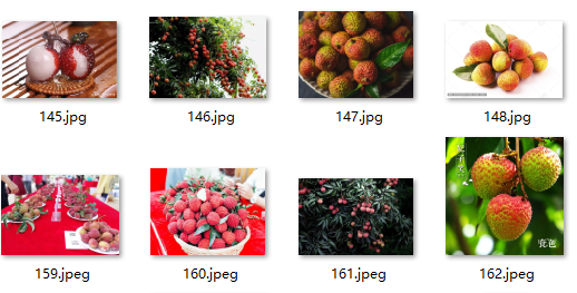
有以下15类：哈密瓜、柠檬、桂圆、梨、榴莲、火龙果、猕猴桃、胡萝卜、芒果、苦瓜、草莓、荔枝、菠萝、车厘子、黄瓜。
数据集中的图片的尺寸大小并不统一，所以在进行模型训练以及验证之前，定义了加载数据集的函数。

def data_load(data_dir, test_data_dir, img_height, img_width, batch_size)

 通过传入的img_height, img_width参数，调用TensorFlow函数

def train_ds = tf.keras.preprocessing.image_dataset_from_directory(
        data_dir,
        label_mode='categorical',
        seed=123,
        image_size=(img_height, img_width),
        batch_size=batch_size) 

 将数据集图片全部处理成img_height * img_width的大小即224*224.

2、 模型结构

 一是使用卷积神经网络（CNN）模型进行水果图片的分类，二是探索轻量级神经网络模型MobileNetV2在水果图像分类中的应用。

2.1 CNN结构

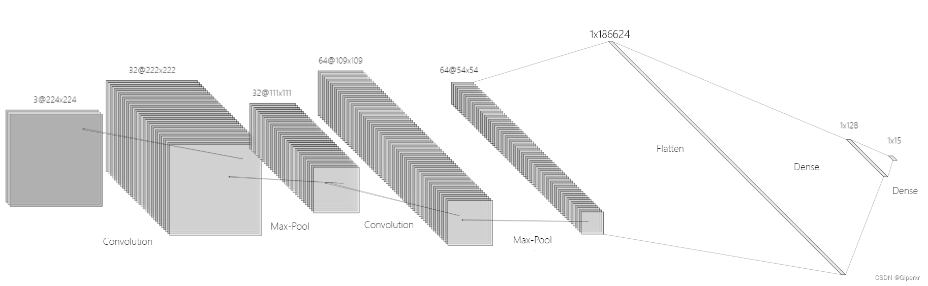
通过TensorFlow构建CNN模型

模型定义函数如下：

def model_load(IMG_SHAPE=(223, 224, 3), class_num=15):
    # 搭建模型
    model = tf.keras.models.Sequential([
        # 对模型做归一化的处理
        tf.keras.layers.experimental.preprocessing.Rescaling(1. / 255, input_shape=IMG_SHAPE),
        # 卷积层
        tf.keras.layers.Conv2D(32, (3, 3), activation='relu'),
        # 池化层
        tf.keras.layers.MaxPooling2D(2, 2),
        # 卷积层
        tf.keras.layers.Conv2D(64, (3, 3), activation='relu'),
        # 池化层
        tf.keras.layers.MaxPooling2D(2, 2),
        # 二维输出转化一维
        tf.keras.layers.Flatten(),
        tf.keras.layers.Dense(128, activation='relu'),
        tf.keras.layers.Dense(class_num, activation='softmax')
    ])
    # 输出模型信息
    model.summary()
    opt = tf.keras.optimizers.SGD(learning_rate=0.005)
    model.compile(optimizer=opt, loss='categorical_crossentropy', metrics=['accuracy'])
    return model

模型介绍：

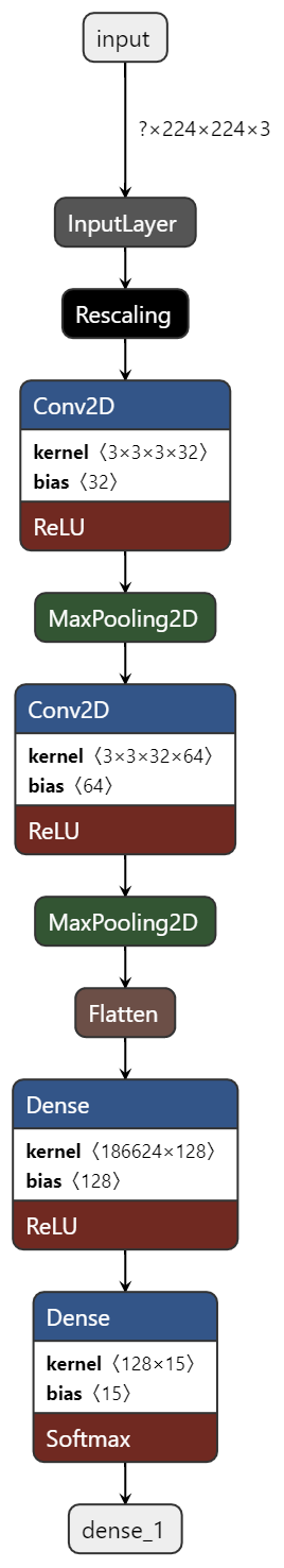
 首先将输入的图片进行归一化处理到0~1之间。然后就是两层卷积层，第一层将通道数由3进行升维到32，第二层则由32升维到64，两层卷积层的卷积核大小都是33，默认步长为1。每层卷积之后都使用Max最大池化，大小22，使用默认步长为2.然后通过Flatten将输出展开到一维长度，随后是一个全连接层，输出到128个神经元。激活函数全部使用的是ReLU。最后一层全连接层，输出映射到15个神经元，因为数据集中是15种水果，采用softMax激活函数，用来预测每个类别的概率。

2.2 MobileNetV2结构

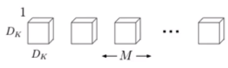
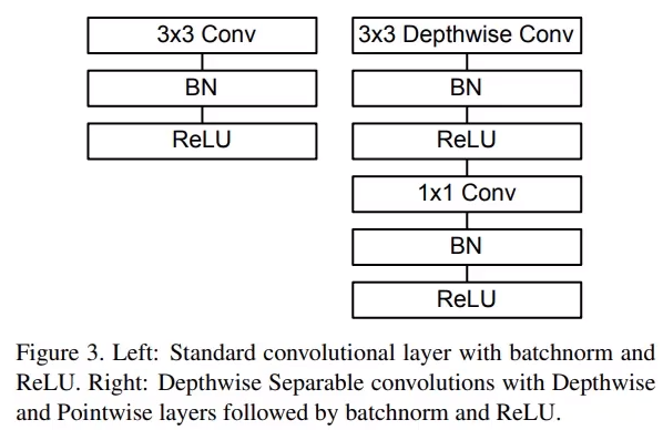
 MobileNet的基本单元是深度可分离卷积，实质是一种可分解卷积操作。可分为两个更小的操作：Depthwise convolution和Pointwise convoluton。
标准的卷积核DkDkM是对与输入通道数M进行卷积操作,N个卷积核。

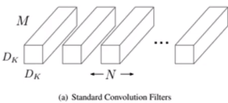
 而MobileNet的Depthwise是对每个输入通道进行分别的卷积 。因为这属于分组卷积，所以在进行卷积操作以后为了减少信息损失，然后再用pointwise convolution也就是1*1的卷积核进行卷积。

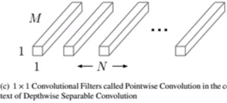
 通过Depthwise convolution和Pointwise convoluton深度可分离卷积以后的整体效果和一个标准卷积差不多，但因为是对不同的通道进行分别卷积，相较于常规的对整体所有通道进行卷积，可以显著的减少计算量，通过pointwise convolution又不损失信息不减少精度，速度更快。

 而MobileNetV2相较于V1的改进，是使用了反向线性残差结构。

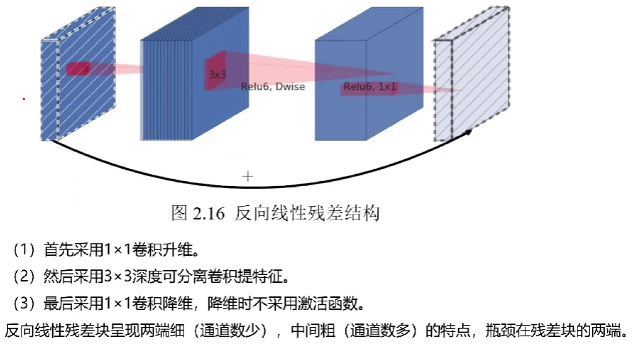
 先采用了1 * 1卷积进行了升维，然后采用3 * 3深度可分离卷积进行特征提取，最后用1 * 1卷积进行降维，降维时不采用激活函数。V2比V1的参数量和计算量会更小、准确率会更高。
模型定义函数如下：

def model_load(IMG_SHAPE=(224, 224, 3), class_num=15):
	#加载预训练的mobilenet模型
    base_model = tf.keras.applications.MobileNetV2(input_shape=IMG_SHAPE,
                                                   include_top=False,
                                                   weights='imagenet')
    base_model.trainable = False
    model = tf.keras.models.Sequential([
        # 进行归一化的处理
        tf.keras.layers.experimental.preprocessing.Rescaling(1. / 127.5, offset=-1, input_shape=IMG_SHAPE),
        # 主干模型
        base_model,
        #全局平均池化
        tf.keras.layers.GlobalAveragePooling2D(),
        # 全连接层
        tf.keras.layers.Dense(class_num, activation='softmax')
    ])
    model.summary()
    model.compile(optimizer='adam', loss='categorical_crossentropy', metrics=['accuracy'])
    return model

模型介绍：

 迁移学习调用了在ImageNet上预训练后的MobileNetV2模型，并去除了顶部的全连接层只留下里面的卷积层和池化层，作为我们的主干模型。冻结了主干模型的参数以适应我们后面自己添加的全连接层的训练，可以加快训练速度。

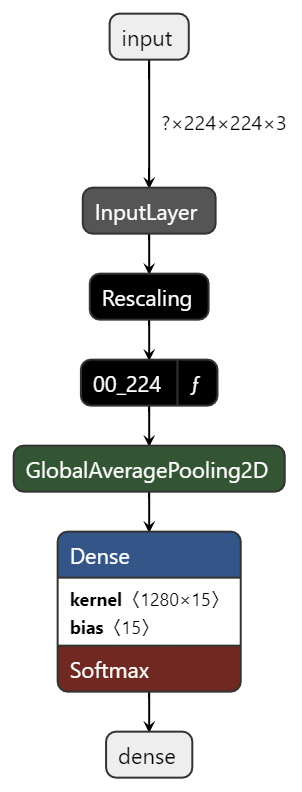
 整个模型先进行归一化，映射到-1~1之间，然后通过我们的主干模型，接着是全局平均池化转化为固定长度的向量。然后就是一个全连接层，映射到class_num个神经元上，也就是我们的水果种类的数量15，通过softmax激活函数预测每个水果类别的概率。

三、 实验结果

1、 CNN训练过程及分析

 除了定义数据集加载函数data_load和模型构建函数model_load外，还定义了showAccuracyAndLoss(history)用来从history中提取模型训练集和验证集的准确率和误差损失，绘制训练过程中的loss和accuracy曲线图。

def data_load(data_dir, test_data_dir, img_height, img_width, batch_size)
def model_load(IMG_SHAPE=(224, 224, 3), class_num=15)
def show_loss_acc(history)

 在train(epochs)函数中调用history = model.fit(train_ds, validation_data=val_ds, epochs=epochs)进行训练，通过model.save("models/cnn_fv.h5")保存为模型文件。

 定义了test_cnn()函数通过保存的模型文件对验证集进行验证，并通过showHM绘制heatmap热力图。
 先使用sgd随机梯度下降优化器和categorical_crossentropy
多分类交叉熵损失函数，epcoh=10进行训练，默认学习率0.01。

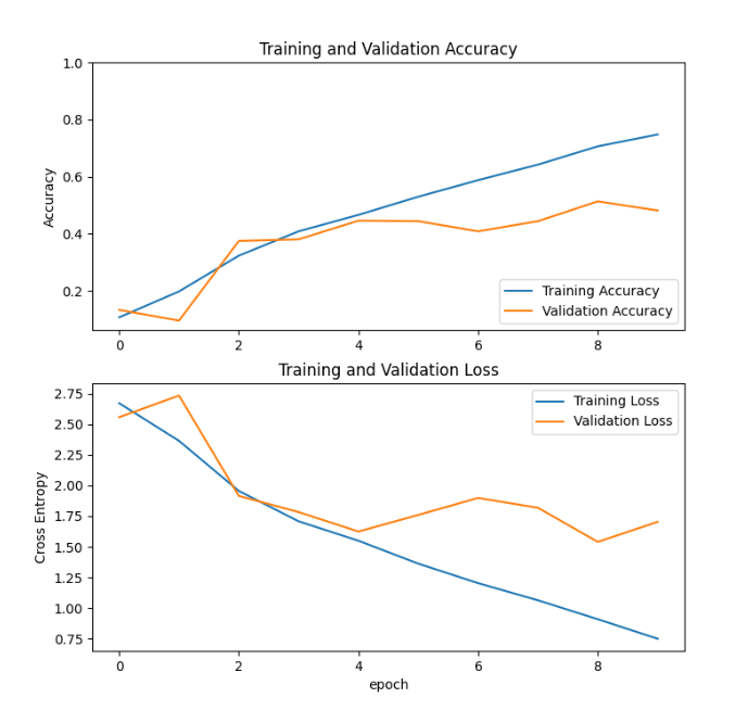
 在第10轮时训练集的准确率只有74%，明显训练轮次过少，调整epoch=25重新训练。

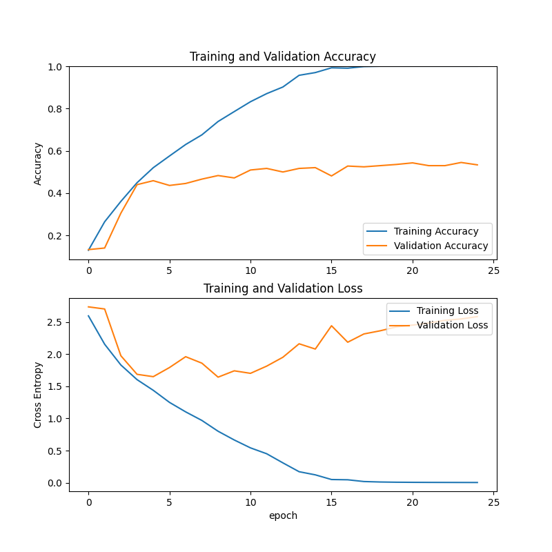
 观察曲线，在18轮以后，训练集的准确率就已经达到了100%，而测试集上的准确率只有50%，随着轮次的增加，测试集上的交叉熵损失值也在增加，发生过拟合。

 测试集的热力图表现出来的准确率也比较差。
 调整学习率，由0.01降为0.05，其它不变，重新训练。

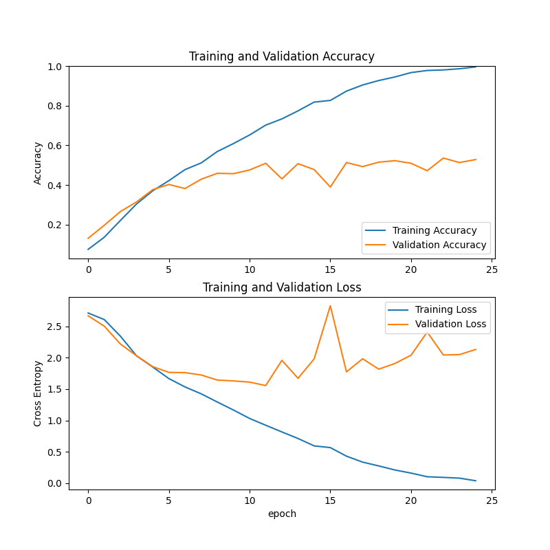
 效果不佳。继续降低学习率为0.001，epoch增加到40，重新训练。

 相较于最初的0.01学习率，测试集上的交叉熵损失在2一下，更低了一点，但是测试集上的准确率还是没有得到很大的提高。

 改变优化器，使用Adam优化器，epoch=40，其它保持不变，学习率默认0.01

 在第10轮时对于训练集的准确率就已经100%，而测试集的交叉熵损失反而达到4以上，比使用sgd优化器时的过拟合更加严重。

 尝试调整CNN网络结构。

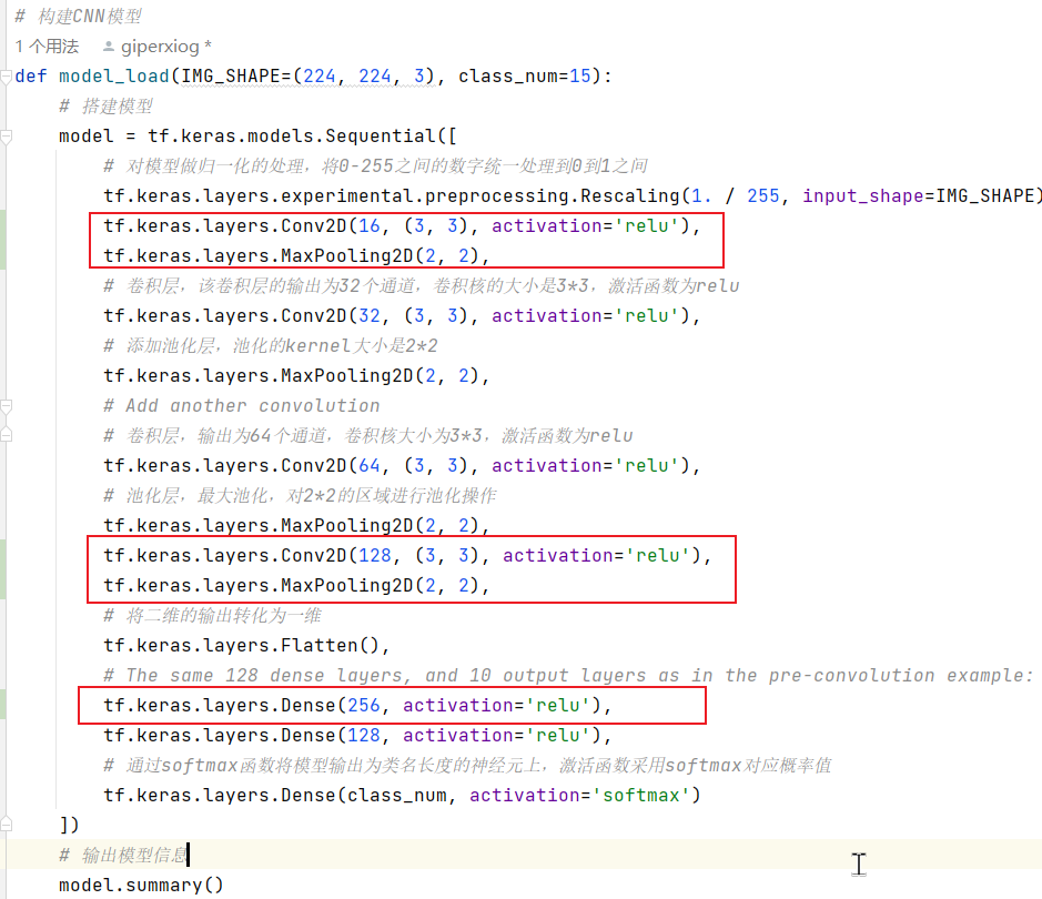
 首尾增加2个卷积层池化层，Flatten展开一维后增加1个全连接层，训练70轮，使用sgd优化器和多分类交叉熵损失函数，效果不理想。

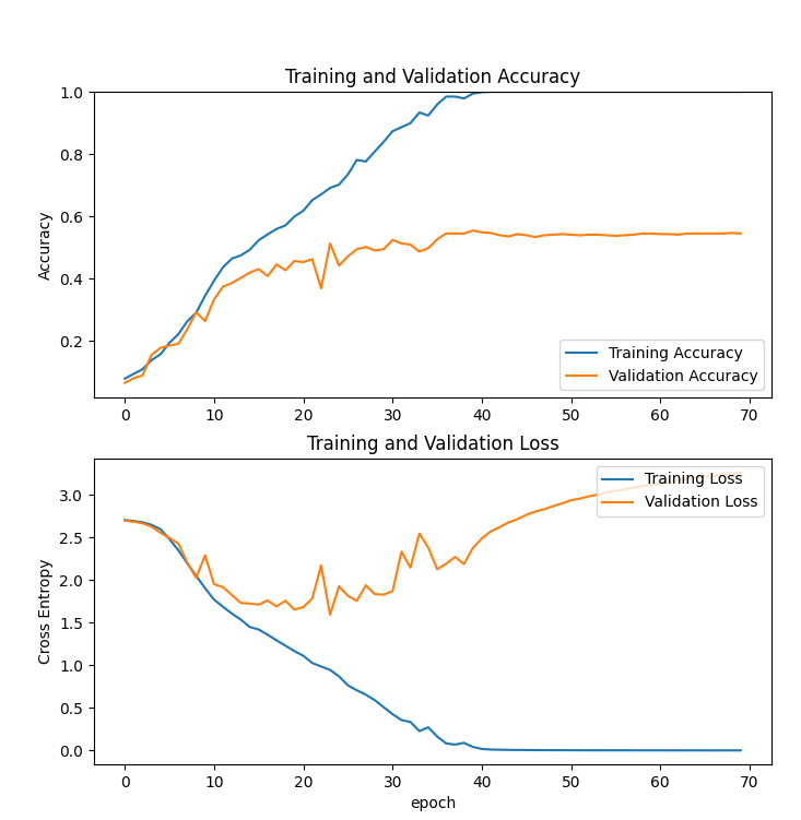
 排查原因，首要原因是数据集的问题，对于像荔枝的数据集，在我们这个模型中预测出来的草莓的概率反而比荔枝更高。查看数据集图片发现这个数据集样本量不够大，荔枝只有156张图片，而且有剥开皮的、还没熟透绿色的、照片调色过艳的，类型过杂图片过少造成预测准确率低。

 利用tensorFlow的ImageDataGenerator对训练集进行数据增强，加上原来的数据集部分，扩大为原来的5倍。

datagen = ImageDataGenerator(
    rotation_range=40,  # 随机旋转角度范围
    width_shift_range=0.2,  # 随机水平平移范围(相对于图片宽度)
    height_shift_range=0.2,  # 随机竖直平移范围(相对于图片高度)
    shear_range=0.2,  # 随机裁剪
    zoom_range=0.2,  # 随机缩放
    horizontal_flip=True,  # 随机水平翻转
    vertical_flip=True,  # 随机竖直翻转
    fill_mode='nearest')  # 填充模式

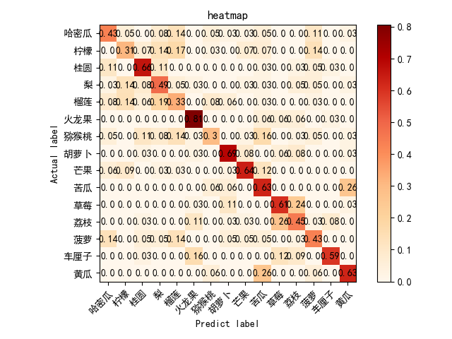
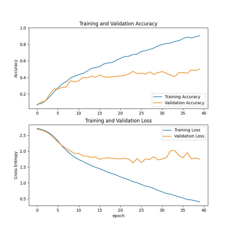
 使用最早定义的CNN网络，epoch=15，sgd优化器和多分类交叉熵损失函数，训练结果如下：

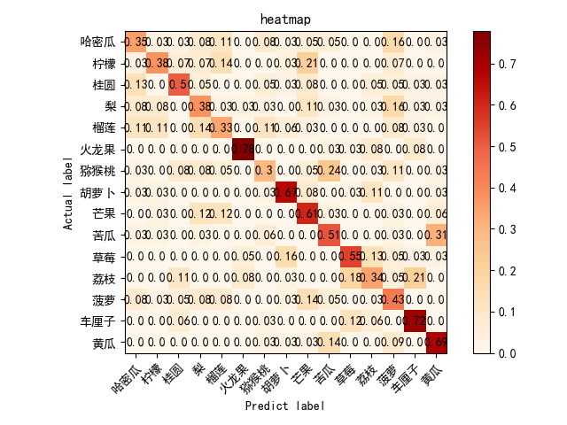
 使用原始的测试集测试后的热力图：

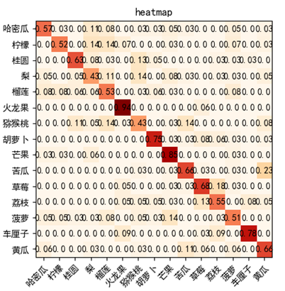
 对数据增强后的测试集进行测试，测试结果热力图：

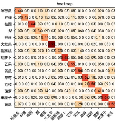
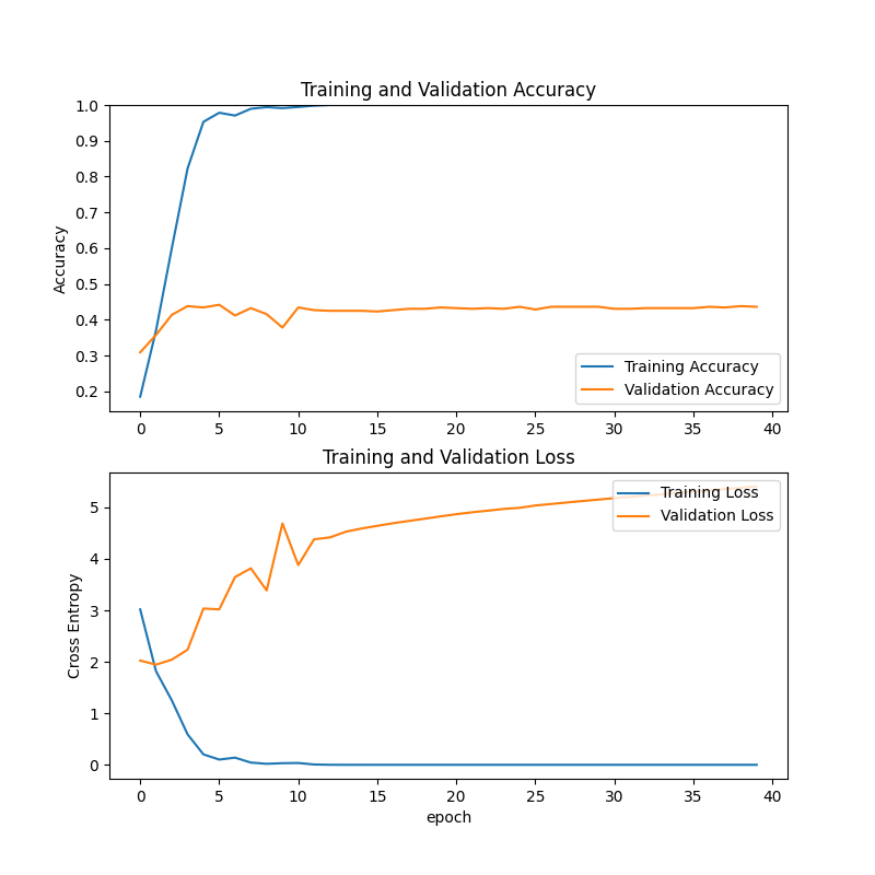
2、 MobileNetV2训练过程及分析

 使用adam优化器和sgd随机梯度下降优化器和categorical_cr ossentropy多分类交叉熵损失函数，默认学习率0.01，epoch=10进行训练。

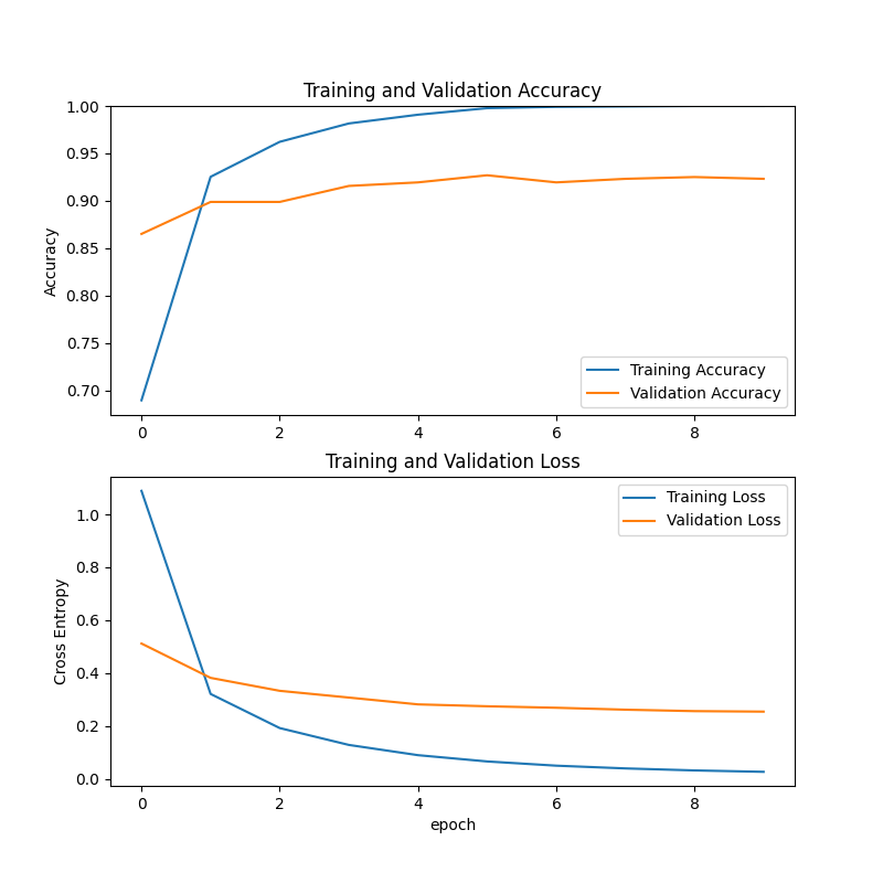
 可以观察到在第6轮训练时，训练集上的准确率就已经达到了100%，而且测试集上的准确率也有90%以上，交叉熵损失达到0.5以下。训练效果非常好。
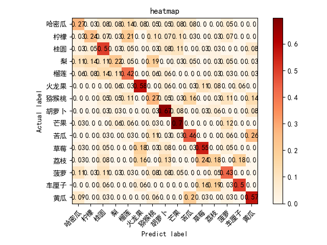
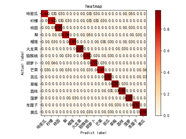
 对原始测试集测试热力图如下：

 对数据增强后的测试集，测试热力图如下：

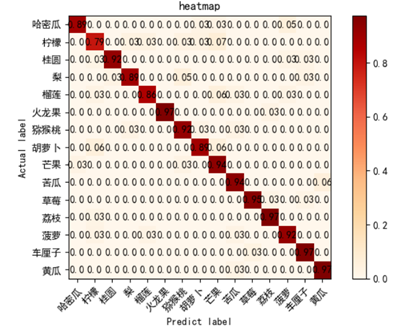
 相比原测试集，准确率只有几类水果稍微下降。

 由此得知，相比较于从头开始训练一个自己的CNN模型，利用迁移学习使用预训练过的MobileNetV2作为主干，利用它在ImageNet上学到的特征，在此基础上进行微调适应自己的数据集，可以显著降低训练时间和成本，大大提高准确度。

四、总结

 在本项目中着重探索了利用深度学习模型进行水果图像分类的方法。具体而言包括使用卷积神经网络（CNN）模型进行水果图片的分类和探索轻量级神经网络模型MobileNetV2在水果图像分类中的应用。

 在第一项任务中，使用TensorFlow构建了一个简单的CNN模型，并通过调整模型参数来提高准确率。在实验过程中发现由于数据集的问题，训练结果并不理想，测试集上的准确率低于预期，同时出现了过拟合的情况。针对这个问题，从优化器、学习率和训练轮次等方面入手，对模型进行了改进和调整。但是由于数据集本身的局限性，改进效果并不显著。后续对数据集进行数据增强，效果相对右改善。因此使用迁移学习中的MobileNetV2模型进行图像分类。

 在第二项任务中，使用预训练的MobileNetV2模型作为主干模型，并对其进行微调以适应自己的数据集。通过这种方法成功地提高了分类准确率。 迁移学习对于解决小规模数据集上的图像分类问题具有重要意义。