利用Tensorflow进行自然语言处理（NLP）系列之二高级Word2Vec

 

       本篇也同步笔者另一博客上（https://blog.csdn.net/qq_37608890/article/details/81530542）

一、概述

在上一篇中，我们介绍了Word2Vec即词向量，对于Word Embeddings即词嵌入有了些基础，同时也阐述了Word2Vec算法的两个常见模型 ：Skip-Gram模型和CBOW模型，本篇会对两种算法做出比较分析并给出其扩展模型-GloVe模型。

 首先，我们将比较下原Skip-gram算法和优化后的新Skip-gram算法情况。对比下Skip-gram与CBOW之间的差异以及两者随迭代次数变化而表现出的不同，利用现有资料，分析一下哪种方法更有利于工作的开展。

其次， 讨论一些有助于提高工作效率的Word2Vec的扩展方法。在学习的过程中，Word2Vec扩展方法涉及负例采样、忽略无效信息等等。当然，还会涉及到一种新的词嵌入技术---Global Vectors（GloVe）及GloVe与Skip-gram和CBOW的比较。

最后，将学习如何使用Word2VEC来解决现实世界的问题：文档分类。

二、原始Skip-gram模型优化前后比较

1、理论说明

         原始Skip-gram模型实际是因为没有中间隐含层（Hidden Layers），而是使用两个不同的embedding 层（嵌入层）或projection层（投影层），且定义了由嵌入层本身派生的代价函数。这里可以对原始Skip-gram和改进后的Skip-gram模型图做个对比。图2-1 是原始Skip-gram模型图，图2-2是改进后的Skip-gram模型图（在上一篇系列一中也有出现）。

 

       

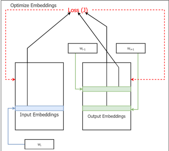
                图2-1 不含隐藏层的原始Skip-gram模型图

 

 

                       图2-2 含有隐含层的改进型Skip-gram模型图

 

2、Tensorflow实施对比

       由于原始Skip-gram模型不含有隐藏层，所以我们无法像上一篇实现的版本那样简单，因为这里的损失函数需要利用TensorFlow手工编制，不像改进版的那样可以直接使用内置函数。实际上就是，没有隐藏层的无法通过Softmax weights和Softmax biases去计算自身的loss。这样在代码实现过程中，主要有两处需要注意，一是 定义模型参数和其他变量；二是 模型计算。

  相关数据及步骤与上一篇（系列之一）一样  ，这里重点给出二者的不同之处、以及随Iterations变化的对比图。

2.1定义模型参数和其他变量

     原始Skip-gram实现的代码

# Variables
 
# Embedding layers, contains the word embeddings
# We define two embedding layers
# in_embeddings is used to lookup embeddings corresponding to target words (inputs)
in_embeddings = tf.Variable(
    tf.random_uniform([vocabulary_size, embedding_size], -1.0, 1.0)
)
# out_embeddings is used to lookup embeddings corresponding to contect words (labels)
out_embeddings = tf.Variable(
    tf.random_uniform([vocabulary_size, embedding_size], -1.0, 1.0)

 改进（或者优化）后的Skip-gram实现的代码   

# Variables
 
# Embedding layer, contains the word embeddings
embeddings = tf.Variable(tf.random_uniform([vocabulary_size, embedding_size], -1.0, 1.0))
 
# Softmax Weights and Biases
softmax_weights = tf.Variable(
    tf.truncated_normal([vocabulary_size, embedding_size],
                        stddev=0.5 / math.sqrt(embedding_size))
)
softmax_biases = tf.Variable(tf.random_uniform([vocabulary_size],0.0,0.01)

  

2.2   模型计算方面 --Defining the Model Computations

     原始Skip-gram实现的代码

    

# 1. Compute negative sampels for a given batch of data
# Returns a [num_sampled] size Tensor
negative_samples, _, _ = tf.nn.log_uniform_candidate_sampler(train_labels, num_true=1, num_sampled=num_sampled, 
                                                           unique=True, range_max=vocabulary_size)
# 2. Look up embeddings for inputs, outputs and negative samples.
in_embed = tf.nn.embedding_lookup(in_embeddings, train_dataset)
out_embed = tf.nn.embedding_lookup(out_embeddings, tf.reshape(train_labels,[-1]))
negative_embed = tf.nn.embedding_lookup(out_embeddings, negative_samples) 
 
# 3. Manually defining negative sample loss
# As Tensorflow have a limited amount of flexibility in the built-in sampled_softmax_loss function,
# we have to manually define the loss fuction.
 
# 3.1. Computing the loss for the positive sample
# Exactly we compute log(sigma(v_o * v_i^T)) with this equation
loss = tf.reduce_mean(
  tf.log(
      tf.nn.sigmoid(
          tf.reduce_sum(
              tf.diag([1.0 for _ in range(batch_size)])*
              tf.matmul(out_embed,tf.transpose(in_embed)),
          axis=0)
      )
  )      
)
 
# 3.2. Computing loss for the negative samples
# We compute sum(log(sigma(-v_no * v_i^T))) with the following
# Note: The exact way this part is computed in TensorFlow library appears to be
# by taking only the weights corresponding to true samples and negative samples
# and then computing the softmax_cross_entropy_with_logits for that subset of weights.
# More infor at: https://github.com/tensorflow/tensorflow/blob/r1.8/tensorflow/python/ops/nn_impl.py
# Though the approach is different, the idea remains the same
loss += tf.reduce_mean(
  tf.reduce_sum(
      tf.log(tf.nn.sigmoid(-tf.matmul(negative_embed,tf.transpose(in_embed)))),
      axis=0
  )
)
 
# The above is the log likelihood. 
# We would like to transform this to the negative log likelihood
# to convert this to a loss. This provides us with
# L = - (log(sigma(v_o * v_i^T))+sum(log(sigma(-v_no * v_i^T))))
loss *= -1.0

 

   改进（或优化）的Skip-gram实现代码       

# Model.
# Look up embeddings for a batch of inputs.
embed = tf.nn.embedding_lookup(embeddings, train_dataset)
 
# Compute the softmax loss, using a sample of the negative labels each time.
loss = tf.reduce_mean(
    tf.nn.sampled_softmax_loss(
        weights=softmax_weights, biases=softmax_biases, inputs=embed,
        labels=train_labels, num_sampled=num_sampled, num_classes=vocabulary_size)

2.3、 原始Skip-gram和改进Skip-gram的对比

        二者对比实现代码         

# Load the skip-gram losses from the calculations we did in Chapter 3
# So you need to make sure you have this csv file before running the code below
skip_loss_path = os.path.join('..','ch3','skip_losses.csv')
with open(skip_loss_path, 'rt') as f:
    reader = csv.reader(f,delimiter=',')
    for r_i,row in enumerate(reader):
        if r_i == 0:
            skip_gram_loss =  [float(s) for s in row]
 
 
pylab.figure(figsize=(15,5))  # figure in inches
 
# Define the x axis
x = np.arange(len(skip_gram_loss))*2000
  
# Plot the skip_gram_loss (loaded from chapter 3)
pylab.plot(x, skip_gram_loss, label="Skip-Gram (Improved)",linestyle='--',linewidth=2)    
# Plot the original skip gram loss from what we just ran
pylab.plot(x, skip_gram_loss_original, label="Skip-Gram (Original)",linewidth=2)
 
# Set some text around the plot
pylab.title('Original vs Improved Skip-Gram Loss Decrease Over Time',fontsize=24)
pylab.xlabel('Iterations',fontsize=22)
pylab.ylabel('Loss',fontsize=22)
pylab.legend(loc=1,fontsize=22)
 
# use for saving the figure if needed
pylab.savefig('loss_skipgram_original_vs_impr.jpg')
pylab.show()

   输出的对比图

         

                             图2-3 The original skip-gram algorithm versus the improved skip-gram algorithm

          从图2-3中的对比，我们不难看出，含有隐藏层的Skip-grm算法比没有隐藏层的Skip-gram算法表现更佳，同时也显示在深度Word2Vec模型处理方面改进后的Skip-gram算法表现更优。

三、Skip-gram模型和CBOW模型比较分析

1、区别

      图2-4和图2-5分别给出了Skip-gram、CBOW模型实施图（在上一篇系列之一中也提到过）。

      像图中显示的那样，给定上下文和目标单词，Skip-gram模型只关注单个输入/输出元组中的目标词和上下文的单个单词，而CBOW则关注目标单词和单个样本中上下文的所有单词。例如 ，短语“狗正对邮递员狂叫”，Skip-gram给出的输入/输出元组是以["dog", "at"]的形式出现，而CBOW则是[["dog","barked","the","mailman"],"at"]。因此，在给定数据集中，对于指定单词的上下文而言，CBOW比Skip-gram会获取更多的信息。下面看下这种差异如何影响两种算法的性能。

 

 

 

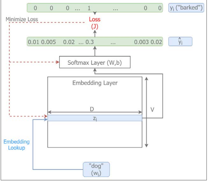
                                  图2-4 Skip-gram模型实施图

 

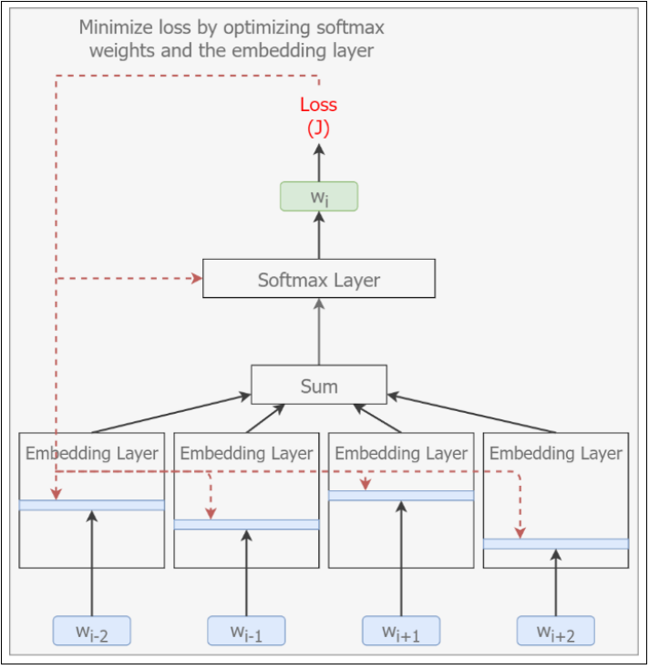
                                  图2-5 CBOW模型实施图

2、性能比较

     现在让我们画出上一篇利用SKip-gram和CBOW算法进行的模型训练任务中的损失随在时间上的表现情况，来看下哪个算法的损失函数下降更快。详见图2-6所示。

     实现代码      

# Load the skip-gram losses from the calculations we did in Chapter 3
# So you need to make sure you have this csv file before running the code below
cbow_loss_path = os.path.join('..','ch3','cbow_losses.csv')
with open(cbow_loss_path, 'rt') as f:
    reader = csv.reader(f,delimiter=',')
    for r_i,row in enumerate(reader):
        if r_i == 0:
            cbow_loss =  [float(s) for s in row]
 
pylab.figure(figsize=(15,5))  # in inches
 
# Define the x axis
x = np.arange(len(skip_gram_loss))*2000
 
# Plot the skip_gram_loss (loaded from chapter 3)
pylab.plot(x, skip_gram_loss, label="Skip-Gram",linestyle='--',linewidth=2)    
# Plot the cbow_loss (loaded from chapter 3)
pylab.plot(x, cbow_loss, label="CBOW",linewidth=2)
 
# Set some text around the plot
pylab.title('Skip-Gram vs CBOW Loss Decrease Over Time',fontsize=24)
pylab.xlabel('Iterations',fontsize=22)
pylab.ylabel('Loss',fontsize=22)
pylab.legend(loc=1,fontsize=22)
 
# use for saving the figure if needed
pylab.savefig('loss_skipgram_vs_cbow.png')
pylab.show()

输出结果

           

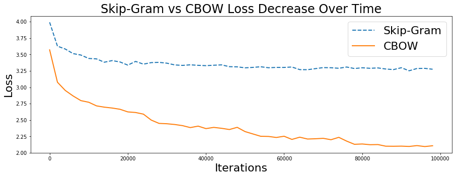
                                                             图2-6  Loss decrease: skip-gram versus CBOW

3、相关分析       

如图2-6所示，与Skip-gram模型相比，CBOW模型的损失下降更快，进一步能够获得更多给定输入-输出元组下目标词的上下文信息。然而，模型损失自身还是足以充分度量模型的性能，因为训练数据过度拟合时损失可能迅速减少。所以，这里再通过一个可视化的角度去检查学习嵌入，以使得Skip-gram模型和CBOW模型在语义上有更显著的区别。这里还是使用比较流行的可视化技术：t-Distributed Stochastic Neighbor Embedding (t-SNE)。

      这里给出部分代码和最终输出结果

       Plotting the Embeddings    

def plot_embeddings_side_by_side(sg_embeddings, cbow_embeddings, sg_labels, cbow_labels):
  ''' Plots word embeddings of skip-gram and CBOW side by side as subplots
  '''
  # number of clusters for each word embedding 
  # clustering is used to assign different colors as a visual aid
  n_clusters = 20 
    
  # automatically build a discrete set of colors, each for cluster
  print('Define Label colors for %d',n_clusters)
  label_colors = [pylab.cm.spectral(float(i) /n_clusters) for i in range(n_clusters)]
  
  # Make sure number of embeddings and their labels are the same
  assert sg_embeddings.shape[0] >= len(sg_labels), 'More labels than embeddings'
  assert cbow_embeddings.shape[0] >= len(cbow_labels), 'More labels than embeddings'
  
  print('Running K-Means for skip-gram')
  # Define K-Means
  sg_kmeans = KMeans(n_clusters=n_clusters, init='k-means++', random_state=0).fit(sg_embeddings)
  sg_kmeans_labels = sg_kmeans.labels_
  sg_cluster_centroids = sg_kmeans.cluster_centers_
 
  print('Running K-Means for CBOW')
  cbow_kmeans = KMeans(n_clusters=n_clusters, init='k-means++', random_state=0).fit(cbow_embeddings)
  cbow_kmeans_labels = cbow_kmeans.labels_
  cbow_cluster_centroids = cbow_kmeans.cluster_centers_
    
  print('K-Means ran successfully')
 
  print('Plotting results')
  pylab.figure(figsize=(25,20))  # in inches
 
  # Get the first subplot
  pylab.subplot(1, 2, 1) 
 
  # Plot all the embeddings and their corresponding words for skip-gram
  for i, (label,klabel) in enumerate(zip(sg_labels,sg_kmeans_labels)):
    center = sg_cluster_centroids[klabel,:]
    x, y = cbow_embeddings[i,:]
    
    # This is just to spread the data points around a bit
    # So that the labels are clearer
    # We repel datapoints from the cluster centroid
    if x < center[0]:
        x += -abs(np.random.normal(scale=2.0))
    else:
        x += abs(np.random.normal(scale=2.0))
        
    if y < center[1]:
        y += -abs(np.random.normal(scale=2.0))
    else:
        y += abs(np.random.normal(scale=2.0))
        
    pylab.scatter(x, y, c=label_colors[klabel])    
    x = x if np.random.random()<0.5 else x + 10
    y = y if np.random.random()<0.5 else y - 10
    pylab.annotate(label, xy=(x, y), xytext=(0, 0), textcoords='offset points',
                   ha='right', va='bottom',fontsize=16)
  pylab.title('t-SNE for Skip-Gram',fontsize=24)
 
  # Get the second subplot
  pylab.subplot(1, 2, 2)  
 
  # Plot all the embeddings and their corresponding words for CBOW
  for i, (label,klabel) in enumerate(zip(cbow_labels,cbow_kmeans_labels)):
    center = cbow_cluster_centroids[klabel,:]
    x, y = cbow_embeddings[i,:]  
    
    # This is just to spread the data points around a bit
    # So that the labels are clearer
    # We repel datapoints from the cluster centroid
    if x < center[0]:
        x += -abs(np.random.normal(scale=2.0))
    else:
        x += abs(np.random.normal(scale=2.0))
        
    if y < center[1]:
        y += -abs(np.random.normal(scale=2.0))
    else:
        y += abs(np.random.normal(scale=2.0))
        
    pylab.scatter(x, y, c=label_colors[klabel])  
    x = x if np.random.random()<0.5 else x + np.random.randint(0,10)
    y = y + np.random.randint(0,5) if np.random.random()<0.5 else y - np.random.randint(0,5)
    pylab.annotate(label, xy=(x, y), xytext=(0, 0), textcoords='offset points',
                   ha='right', va='bottom',fontsize=16)
 
  pylab.title('t-SNE for CBOW',fontsize=24)
  # use for saving the figure if needed
  pylab.savefig('tsne_skip_vs_cbow.png')
  pylab.show()
 
# Run the function
sg_words = [reverse_dictionary[i] for i in sg_selected_ids]
cbow_words = [reverse_dictionary[i] for i in cbow_selected_ids]
plot_embeddings_side_by_side(sg_two_d_embeddings, cbow_two_d_embeddings, sg_words,cbow_words)

      最终输出结果（含对比图片） 。

       说明：实际输出图片是两张并排显示的，笔者为了尽可能让图片显示清楚又单独做的截图。

 

Define Label colors for %d 20
Running K-Means for skip-gram
Running K-Means for CBOW
K-Means ran successfully

 

         

           

 

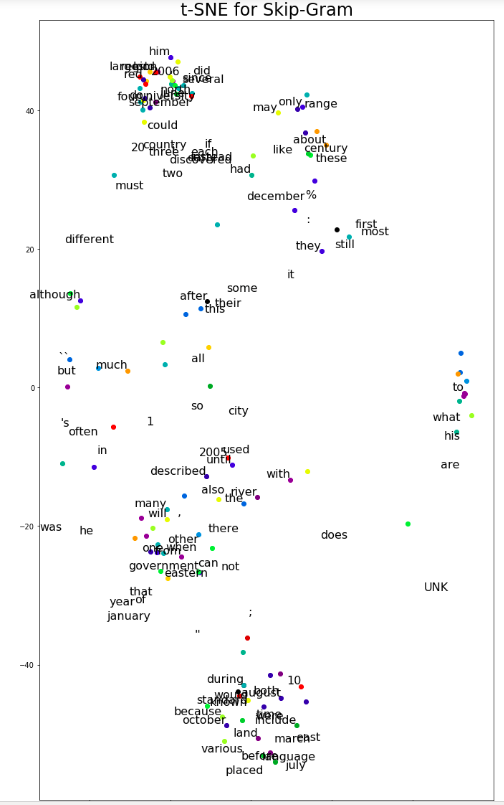
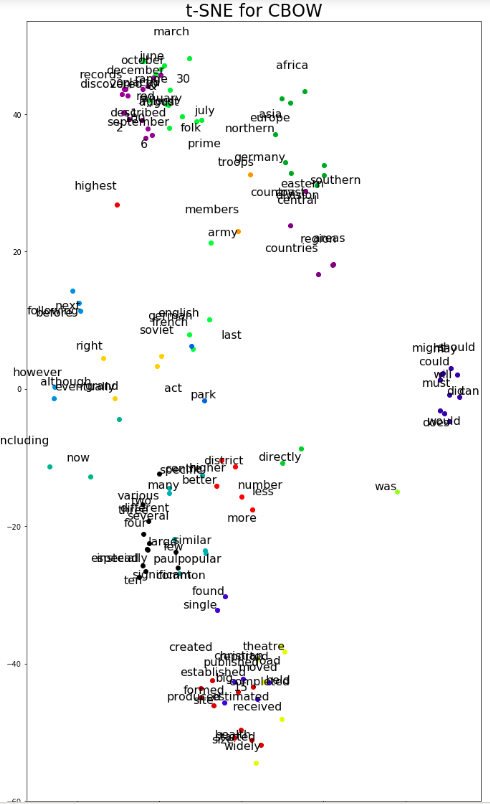
        由图中所示，我们可以发现，CBOW模型对单词的聚类分析效果更佳，所以，可以说，在这部分例子中，CBOW 模型比Skip-gram模型更优。

4、CBOW及其扩展的对比

    这里本来想展开分析，但考虑的本文篇幅问题，就不做过多解读，简要给出CBOW、CBOW(Unigram)、CBOW (Unigram+Subsampling)之间的对比，网上还没找到关于三者之间对比的深入解读，感兴趣的读者可以细看Thushan Ganegedara写的《Natural Language Processing with TensorFlow》。

       基于负采样例和子采样例损失三者的对比图         

 

pylab.figure(figsize=(15,5))  # in inches
 
# Define the x axis
x = np.arange(len(skip_gram_loss))*2000
 
# Plotting standard CBOW loss, CBOW loss with unigram sampling and
# CBOW loss with unigram sampling + subsampling here in one plot
pylab.plot(x, cbow_loss, label="CBOW",linestyle='--',linewidth=2)
pylab.plot(x, cbow_loss_unigram, label="CBOW (Unigram)",linestyle='-.',linewidth=2,marker='^',markersize=5)
pylab.plot(x, cbow_loss_unigram_subsampled, label="CBOW (Unigram+Subsampling)",linewidth=2)
 
# Some text around the plots
pylab.title('Original CBOW vs Various Improvements Loss Decrease Over-Time',fontsize=24)
pylab.xlabel('Iterations',fontsize=22)
pylab.ylabel('Loss',fontsize=22)
pylab.legend(loc=1,fontsize=22)
 
# Use for saving the figure if needed
pylab.savefig('loss_cbow_vs_all_improvements.png')
pylab.show()

 

   输出结果

      

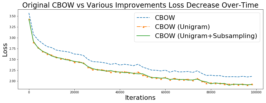
    这里发现一个有意思的现象，CBOW(Unigram)和CBOW (Unigram+Subsampling)给出了几乎一样的损失值。然而，这不应该被错误地理解为Subsampling在学习问题上优势有缺失。这种特殊现象产生的原因如下：和二次采样（Subsampling）一样，我们去掉了一些无效的单词（这些单词具有信息意义），引起文本质量上升（就信息质量而言）。这样就反过来使得学习的问题变得更加困难。在之前的问题设置中，词向量本来有机会在优化处理中对无效单词（就信息意义而言）加以利用处理，而现在新的问题设置中，这些机会已经非常小了，这就带来更大的损失，但语义上的声音词向量还在。

四、GloVe模型

         学习单词向量的方法分为两类：  基于全局矩阵分解的方法或基于局部上下文窗口的方法。潜在语义分析（LSA）是一种基于全局矩阵分解的方法，Skip-gram和CBOW是基于局部上下文窗口的方法。作为一种文档 析技术，LSA将文档中的单词映射成一种“概念”，这“概念”在文档中以一种常见的单词模式呈现出来。而基于全局矩阵分解的方法则有效地利用了语料库的全局统计（例如，全局范围内单词的共现情形），但这种在词类类比任务中效果一般。另一方面，基于上下文窗口的方法已在词语类比任务中表现良好，但却没有充分使用语料库的全局统计，这就为后续的改进工作留出了空间。

        1、通过例子增强对GloVe的理解

           在对GloVe进行实施之前，我们先看个例子，增强对于GloVe的理解。

           1）、这里有两个单词 : i="dog" 和 j ="cat".

           2)、   定义任一探测词k；

           3）、    用Pik 单词i和单词k 表示单词i和单词k同时出现的概率 ，Pjk分别表示单词j和单词k同时出现的概率。

         现在看下，在k取不同值的情况下pik/pjk的变化情况。

           对于k=“bark”而言，这里k与i一起出现的概率很高，与j同时出现的可能性极小，因此Pik/Pjk >>1。

            当k="purr"时，k不太可能出现在i附近，则Pik较小；而k却与j高度相关，则Pjk值较高。所以 Pik/Pjk的近似值为0。

           对于K=“PET”这样的词，它与I和J都有很强的关系，或者K=“politics”，与两者都具有最小的相关性，所以这时我们得到：  Pik/Pjk的值为1。

         可以看出，实体Pik/Pjk是一种通过近距离两个词的共现频率去度量二者的关系一种衡量方法。因此，它对于学习好的词向量是一种不错的备选方法。那么，下定义一个损失函数就成为我们开启相关工作的不错的起点，

          由

​

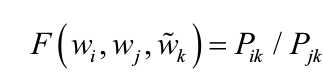
               有关资料经过认真推导得到如下损失函数。

 

​

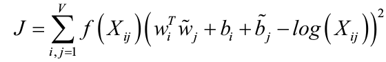
   2、GloVe模型实施

    2.1 数据集

       数据与上一篇使用的数据一样，即dataset.

2.2 相关步骤

         与上一篇Skip-gram模型流程类似。

•      用NLTK对数据进行预处理；

•      建立相关Dictionaries；

•      给出数据的Batches；

•       明确超参数、输出样本、输入样本、模型参数及其他变量；

•        确定模型计算、计算单词相似性；

•        模型优化、执行；

    2.3 给出部分代码及最终输出结果

          模型执行代码           

num_steps = 100001
glove_loss = []
 
average_loss = 0
with tf.Session(config=tf.ConfigProto(allow_soft_placement=True)) as session:
    
    tf.global_variables_initializer().run()
    print('Initialized')
    
    for step in range(num_steps):
        
        # generate a single batch (data,labels,co-occurance weights)
        batch_data, batch_labels, batch_weights = generate_batch(
            batch_size, skip_window) 
        
        # Computing the weights required by the loss function
        batch_weights = [] # weighting used in the loss function
        batch_xij = [] # weighted frequency of finding i near j
        
        # Compute the weights for each datapoint in the batch
        for inp,lbl in zip(batch_data,batch_labels.reshape(-1)):     
            point_weight = (cooc_mat[inp,lbl]/100.0)**0.75 if cooc_mat[inp,lbl]<100.0 else 1.0 
            batch_weights.append(point_weight)
            batch_xij.append(cooc_mat[inp,lbl])
        batch_weights = np.clip(batch_weights,-100,1)
        batch_xij = np.asarray(batch_xij)
        
        # Populate the feed_dict and run the optimizer (minimize loss)
        # and compute the loss. Specifically we provide
        # train_dataset/train_labels: training inputs and training labels
        # weights_x: measures the importance of a data point with respect to how much those two words co-occur
        # x_ij: co-occurence matrix value for the row and column denoted by the words in a datapoint
        feed_dict = {train_dataset : batch_data.reshape(-1), train_labels : batch_labels.reshape(-1),
                    weights_x:batch_weights,x_ij:batch_xij}
        _, l = session.run([optimizer, loss], feed_dict=feed_dict)
        
        # Update the average loss variable
        average_loss += l
        if step % 2000 == 0:
          if step > 0:
            average_loss = average_loss / 2000
          # The average loss is an estimate of the loss over the last 2000 batches.
          print('Average loss at step %d: %f' % (step, average_loss))
          glove_loss.append(average_loss)
          average_loss = 0
        
        # Here we compute the top_k closest words for a given validation word
        # in terms of the cosine distance
        # We do this for all the words in the validation set
        # Note: This is an expensive step
        if step % 10000 == 0:
          sim = similarity.eval()
          for i in range(valid_size):
            valid_word = reverse_dictionary[valid_examples[i]]
            top_k = 8 # number of nearest neighbors
            nearest = (-sim[i, :]).argsort()[1:top_k+1]
            log = 'Nearest to %s:' % valid_word
            for k in range(top_k):
              close_word = reverse_dictionary[nearest[k]]
              log = '%s %s,' % (log, close_word)
            print(log)
            
    final_embeddings = normalized_embeddings.eval()

 

       输出（给出部分内容，中间删除一部分）

        

Initialized
Average loss at step 0: 9.578778
Nearest to it: karol, burgh, destabilise, armchair, crook, roguery, one-sixth, swains,
Nearest to that: wmap, partake, ahmadi, armstrong, memberships, forza, director-general, condo,
Nearest to has: mentality, vastly, approaches, bulwark, enzymes, originally, privatize, reunify,
Nearest to but: inhabited, potrero, trust, memory, curran, philips, p.m.s, pagoda,
Nearest to city: seals, counter-revolution, tubular, kayaking, central, 1568, override, buckland,
Nearest to this: dispersion, intermarriage, dialysis, moguls, aldermen, alcoholic, codes, farallon,
Nearest to UNK: 40.3, tatsam, jupiter, verify, unequal, berliners, march, 1559,
Nearest to by: functionalists, synthesised, palladius, chiapas, synaptic, sumner, raining, valued,
Nearest to or: amherst, 'mother, epiglottis, wen, stanislaus, trafford, cuticle, reminded,
Nearest to been: 640,961., depression-era, uniquely, mami, 375,000, stickiness, medium-sized, amor,
Nearest to with: anti-statist, pitigliano, branches, reparations, acquittal, frowned, pishpek, left-leaning,
Nearest to be: i-20, kevin, greased, rightly, conductors, hypercholesterolemia, pedro, douaumont,
Nearest to as: gabon, horda, mead, protruding, soundtrack, algeria, 48, macon,
Nearest to at: kambula, tisa, spelled, 130,000, 2008, organisers, |jul_rec_lo_°f, arrows,
Nearest to ,: is, of, its, malton, martinů, retiree, reliant, uri,
Nearest to its: of, ,, galleon, gitlow, rugby-playing, varanasi, fono, clusters,
Average loss at step 2000: 0.739107
Average loss at step 4000: 0.091107
Average loss at step 6000: 0.068614
Average loss at step 8000: 0.076040
Average loss at step 10000: 0.058149
Nearest to it: was, is, that, not, a, in, to, .,
Nearest to that: is, was, the, a, ., ,, to, in,
Nearest to has: is, it, that, a, been, was, to, mentality,
Nearest to but: with, said, trust, mating, not, squamous, war—the, r101,
Nearest to city: of, 's, counter-revolution, the, professed, ., equilibrium, seals,
Nearest to this: is, ., for, in, was, the, a, that,
Nearest to UNK: and, ,, (, in, the, ., ), a,
Nearest to by: the, and, ,, ., in, was, of, a,
Nearest to or: UNK, ,, and, a, cuticle, donnchad, ``, 'mother,
Nearest to been: have, had, to, has, be, was, that, it,
Nearest to with: ,, and, a, the, in, of, for, .,
 
Nearest to by: the, was, ,, in, ., and, a, of,
Nearest to or: (, UNK, ), ``, a, ,, and, with,
Nearest to been: have, has, had, also, be, that, was, to,
Nearest to with: and, ,, a, the, of, in, for, .,
Nearest to be: to, have, can, not, that, from, is, would,
Nearest to as: a, an, ,, such, for, and, is, the,
Nearest to at: of, the, ., in, 's, ,, and, by,
Nearest to ,: and, in, the, ., a, with, of, UNK,
Nearest to its: for, and, their, with, his, ,, the, of,
Average loss at step 92000: 0.019305
Average loss at step 94000: 0.019555
Average loss at step 96000: 0.019266
Average loss at step 98000: 0.018803
Average loss at step 100000: 0.018488
Nearest to it: is, was, also, that, not, has, this, a,
Nearest to that: was, is, to, it, the, a, ., ,,
Nearest to has: it, been, was, had, also, is, that, a,
Nearest to but: which, not, ,, it, with, was, and, a,
Nearest to city: of, 's, the, ., in, is, new, world,
Nearest to this: is, ., was, it, in, for, the, at,
Nearest to UNK: (, and, ), ,, or, a, the, .,
Nearest to by: the, ., was, ,, and, in, of, a,
Nearest to or: UNK, (, ``, a, ), ,, and, with,
Nearest to been: have, has, had, also, be, was, that, to,
Nearest to with: and, ,, a, the, of, in, for, .,
Nearest to be: to, have, can, not, would, from, that, a,
Nearest to as: a, such, an, ,, for, is, and, to,
Nearest to at: of, ., the, in, 's, by, ,, and,
Nearest to ,: and, in, the, ., a, with, UNK, of,
Nearest to its: for, their, and, with, his, ,, to, the,

     

五、Word2Vec解决文档分类

          虽然词嵌入给出了一种非常优雅的学习单词数字化表示方法，但正如我们看到的那样，这些孤立的定量（损失值）和定性（T-SNE嵌入）学习词表示的效用在现实世界的词表示方面是令人不能满意的。字嵌入被用作许多任务的词特征表示，例如图像字幕生成和机器翻译。然而，这些任务涉及组合不同的学习模型（如卷积神经网络（CNNs）和长短时记忆（LSTM）模型或两个LSTM模型），将在后面的篇幅中继续讨论。这里就涉及到在现实世界中词嵌入的实际应用情况，所以，这里给出一个简单的文档分类任务。

            文档分类是NLP中最流行的任务之一，它对于处理海量数据（比如新闻网站、出版商、大学）的人员来说是非常有用的。所以，下面我们使用的来自BBC的新闻文章，每一文件属于以下类别：商业、娱乐、政治、体育或技术。每个类别使用其中的250个文档，词汇量规模为25，000。另外，每个文档都将用一种“<文档> -<ID>”标签来表示。例如，娱乐部的第五十份文件将被表示为“娱乐版-50”。与现实世界中被分析应用的大型文本语料库相比，这是一个非常小的数据集，但这个小的例子可以让我们看到词嵌入的威力。

     1、数据集

           来自BBC新闻：Dataset，给出。

     2、相关步骤

         

•  用NLTK对数据进行预处理；

•      建立相关Dictionaries，包括word到ID、ID到word及单词list（word，frequency）等；

•     用Skip-gram 给出数据的Batches；

•       明确超参数、输出、输入、模型参数及其他变量；

•        计算损失、单词相似性；

•        模型优化、执行CBOW算法模型；

•        利用 t-SNE Results给出可视化结果；

•         执行文档分类。

3、这里给出部分代码和输出结果

     3.1  Running the CBOW Algorithm on Document Data

        

num_steps = 100001
cbow_loss = []
 
config=tf.ConfigProto(allow_soft_placement=True)
# This is an important setting and with limited GPU memory,
# not using this option might lead to the following error.
# InternalError (see above for traceback): Blas GEMM launch failed : ...
config.gpu_options.allow_growth = True
 
with tf.Session(config=config) as session:
    
    # Initialize the variables in the graph
    tf.global_variables_initializer().run()
    print('Initialized')
    
    average_loss = 0
    
    # Train the Word2vec model for num_step iterations
    for step in range(num_steps):
        
        # Generate a single batch of data
        batch_data, batch_labels = generate_batch(data, batch_size, window_size)
        
        # Populate the feed_dict and run the optimizer (minimize loss)
        # and compute the loss
        feed_dict = {train_dataset : batch_data, train_labels : batch_labels}
        _, l = session.run([optimizer, loss], feed_dict=feed_dict)
        
        # Update the average loss variable
        average_loss += l
        
        if (step+1) % 2000 == 0:
            if step > 0:
                average_loss = average_loss / 2000
                # The average loss is an estimate of the loss over the last 2000 batches.
            print('Average loss at step %d: %f' % (step+1, average_loss))
            cbow_loss.append(average_loss)
            average_loss = 0
        
        # Evaluating validation set word similarities
        if (step+1) % 10000 == 0:
            sim = similarity.eval()
            # Here we compute the top_k closest words for a given validation word
            # in terms of the cosine distance
            # We do this for all the words in the validation set
            # Note: This is an expensive step
            for i in range(valid_size):
                valid_word = reverse_dictionary[valid_examples[i]]
                top_k = 8 # number of nearest neighbors
                nearest = (-sim[i, :]).argsort()[1:top_k+1]
                log = 'Nearest to %s:' % valid_word
                for k in range(top_k):
                    close_word = reverse_dictionary[nearest[k]]
                    log = '%s %s,' % (log, close_word)
                print(log)
    
    # Computing test documents embeddings by averaging word embeddings
    
    # We take batch_size*num_test_steps words from each document
    # to compute document embeddings
    num_test_steps = 100
    
    # Store document embeddings
    # {document_id:embedding} format
    document_embeddings = {}
    print('Testing Phase (Compute document embeddings)')
    
    # For each test document compute document embeddings
    for k,v in test_data.items():
        print('\tCalculating mean embedding for document ',k,' with ', num_test_steps, ' steps.')
        test_data_index = 0
        topic_mean_batch_embeddings = np.empty((num_test_steps,embedding_size),dtype=np.float32)
        
        # keep averaging mean word embeddings obtained for each step
        for test_step in range(num_test_steps):
            test_batch_labels = generate_test_batch(test_data[k],batch_size)
            batch_mean = session.run(mean_batch_embedding,feed_dict={test_labels:test_batch_labels})
            topic_mean_batch_embeddings[test_step,:] = batch_mean
        document_embeddings[k] = np.mean(topic_mean_batch_embeddings,axis=0)

输出（给出部分内容）     

Initialized
Average loss at step 2000: 3.914388
Average loss at step 4000: 3.562556
Average loss at step 6000: 3.545086
Average loss at step 8000: 3.549088
Average loss at step 10000: 3.481902
Nearest to .: ,, and, mp3s, friendlies, -, that, documentary, low,
Nearest to i: we, is, appreciate, outsiders, icann, modelling, onslaught, chennai,
Nearest to which: impromptu, israeli, skills, portuguese, ghanaian, lifetime, innocence, paisley,
Nearest to were: are, cryptography, heaped, 836m, 50mg, pervasively, 28,000, past,
Nearest to we: people, they, enormity, i, ranked, is, jacob, are,
Nearest to they: we, softer, to, not, revisions, 27.24, 'template, be,
Nearest to would: will, to, should, alleges, sleepless, jolie, also, could,
Nearest to that: not, about, it, ., change, get, politicians, gartner,
Nearest to had: has, have, was, streets, bulgaria, directory, nestle, binding,
Nearest to said: added, restriction-free, forgiven, breathing, allardyce, intends, vans, he,
Nearest to this: 2005/06, build, connectotel, it, short, greenback, last, diet,
Nearest to he: it, inaccurate, mr, she, '', 102, was, has,
Nearest to not: that, complained, phenomenon, sourced, they, 10.4, cliques, 'template,
Nearest to it: he, there, everyday, that, ``, 6gb, this, did,
Nearest to ,: ., 's, the, sleeves, and, singer/guitarist, legislative, observed,
Nearest to from: for, hermann, in, and, by, jeep, flights, asher,
Testing Phase (Compute document embeddings)
    Calculating mean embedding for document  tech-34  with  100  steps.
    Calculating mean embedding for document  sport-166  with  100  steps.
    Calculating mean embedding for document  sport-87  with  100  steps.
    Calculating mean embedding for document  entertainment-119  with  100  steps.
    Calculating mean embedding for document  business-161  with  100  steps.
    Calculating mean embedding for document  sport-129  with  100  steps.
    Calculating mean embedding for document  tech-145  with  100  steps.
    Calculating mean embedding for document  business-135  with  100  steps.
    Calculating mean embedding for document  sport-206  with  100  steps.
    Calculating mean embedding for document  tech-216  with  100  steps.
    Calculating mean embedding for document  entertainment-216  with  100  steps.
    Calculating mean embedding for document  politics-184  with  100  steps.
    Calculating mean embedding for document  sport-184  with  100  steps.
    Calculating mean embedding for document  sport-45  with  100  steps.
    Calculating mean embedding for document  sport-32  with  100  steps.
    Calculating mean embedding for document  politics-247  with  100  steps.
    Calculating mean embedding for document  business-240  with  100  steps.
    Calculating mean embedding for document  entertainment-98  with  100  steps.
    Calculating mean embedding for document  politics-171  with  100  steps.
    Calculating mean embedding for document  politics-8  with  100  steps.
    Calculating mean embedding for document  business-165  with  100  steps.
    Calculating mean embedding for document  politics-16  with  100  steps.
    Calculating mean embedding for document  business-44  with  100  steps.
    Calculating mean embedding for document  business-215  with  100  steps.
    Calculating mean embedding for document  tech-79  with  100  steps.
    Calculating mean embedding for document  tech-178  with  100  steps.
    Calculating mean embedding for document  entertainment-163  with  100  steps.
    Calculating mean embedding for document  entertainment-196  with  100  steps.
    Calculating mean embedding for document  politics-236  with  100  steps.
    Calculating mean embedding for document  entertainment-1  with  100  steps.
    Calculating mean embedding for document  sport-20  with  100  steps.
    Calculating mean embedding for document  tech-157  with  100  steps.

    3.2   用t-SNE可视化输出结果下图

          

         3.3 文档分类

   

# Create and fit K-means
kmeans = KMeans(n_clusters=5, random_state=43643, max_iter=10000, n_init=100, algorithm='elkan')
kmeans.fit(np.array(list(document_embeddings.values())))
 
# Compute items fallen within each cluster
document_classes = {}
for inp, lbl in zip(list(document_embeddings.keys()), kmeans.labels_):
    if lbl not in document_classes:
        document_classes[lbl] = [inp]
    else:
        document_classes[lbl].append(inp)
for k,v in document_classes.items():    
    print('\nDocuments in Cluster ',k)
    print('\t',v)

    输出

  

Documents in Cluster  0
     ['entertainment-216', 'business-240', 'business-44', 'tech-178', 'business-165', 'tech-238', 'business-171', 'business-144', 'business-107']
 
Documents in Cluster  1
     ['tech-34', 'tech-145', 'business-135', 'sport-206', 'tech-216', 'politics-184', 'politics-247', 'politics-171', 'politics-8', 'politics-78', 'entertainment-163', 'politics-16', 'business-141', 'business-215', 'tech-79', 'tech-157', 'sport-231', 'tech-42', 'politics-197', 'politics-98', 'tech-212']
 
Documents in Cluster  2
     ['sport-166', 'entertainment-119', 'business-161', 'sport-129', 'sport-45', 'entertainment-98', 'entertainment-196', 'politics-236', 'sport-26', 'entertainment-1', 'entertainment-74', 'entertainment-244', 'entertainment-154']
 
Documents in Cluster  3
     ['sport-184']
 
Documents in Cluster  4
     ['sport-87', 'sport-32', 'sport-20']

  

4、简要分析

         从聚类的结果来看效果可能一般，但最起码该模型将文件做了一个较为初步的分类，大体上还算靠谱，至于遇到的部分文件没有被划分到正确的群簇内，是由于相关内容与目前群簇存在一定的内在联系，笔者大体上简单看了下sport-206和tech-34，其他的没来得及全看，各位读者感兴趣的话可以从数据集中仔细查验，这里先不做进一步的说明，以后有时间再回过头看看。

       备注说明：书给出的t-SNE可视化 图片与代码运行的结果不一致，尤其提到tech-42在图中的位置明显相反，至于提到的与sport-50和ertainment-115的分析情况，由于与代码运行有些差异，所以这里就不针对书中的内容做过多的解释，读者感兴趣的话可以自行查验。

六、简要总结

         首先，我们分析了Skip-gram和CBOW算法之间性能上的差异。为了更好地突出二者之间的区别，我们使用了常见的可视化技术--t-SNE，得到了二者之间背后更直观的区别。

        其次，我们开展了词向量（Word2Vec）方面的拓展，并基于Skip-gram和CBOW模型的新算法的性能进行了对比分析。

         接下来，我们对于著名的GloVe模型进行了相关介绍和分析， 由于GloVe模型纳入了全局优化统计，所以在整体性能上得到了很大提升。

       最后，我们开展了一个文档分类方面的分析。

     关于后续篇幅，是开展CNN、RNN、LSTM后再进行文本生成、图片主题词提取、机器翻译还是直接从文本生成开始，目前没定，后续再定。自身水平有限，如有不足之处，请各位网友多指点。

 

近期有些事情要处理，博客更新可能会延迟些。