利用Tensorflow进行自然语言处理(NLP)系列之一Word2Vec
同步笔者CSDN博客(https://blog.csdn.net/qq_37608890/article/details/81513882)。
一、概述
本文将要讨论NLP的一个重要话题:Word2Vec,它是一种学习词嵌入或分布式数字特征表示(即向量)的技术。其实,在开展自然语言处理任务时,一个比较重要的基础工作就是有关词表示层面的学习,因为良好的特征表示所对应的词,能够使得上下午语义内容得以很好地保留和整体串起来。举个例子,在特征表示层面,单词“forest”和单词“oven”是不同的,也很少在类似的上下文中出现,而单词“forest”和单词“jungle”应该是很相似的。
Word2Vec也被称为分布式表示,因为单词的语义是由全表示向量的激活模式获得的,与单个元素的表示向量就形成了对比。
接下来,我们会一步步地提供从传统方法到以现代神经网络为基础的先进方法,针对词表示做进一步说明。我们可以使用T-SNE(一种高维数据的可视化技术)将单词数据集进行可视化,如图1.1所展示的2D样式。显然,相似的词会离的很近。这里初步给大家一个关于Word2Vec的直观认识。
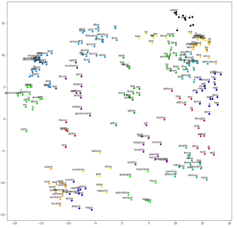
图1-1 一个利用t-SNE进行学习词嵌入可视化例子
关于t-SNE(也就是t-Distributed Stochastic Neighbor Embedding)的内容,可以参考另外一篇文章《从SNE到t-SNE再到LargeVis》,里面作者写挺好的,感兴趣的网友可以详细看下。
二、关于词的表示(Word Representation)或词义(word meaning)的理解
单纯从语言学的角度来讲,词义应该是个偏哲学方面的问题,而不是技术问题,但这里会给出一个比较温和的阐述:词义是一个词传达出的思想或者表达方式。因为NLP的主要目标是能够让机器在语言领域实现人类相似的功能,所以,我们深入研究机器的词表示规则是很明智的。而在计算机领域,任何信息的存储方式都是数字化或者说0和1二进制化的,我们会给所有的字符(包括字母字符,汉字、英语单词等语言文字)一个编码方式。为了实现我们的目标,我们会使用可以分析指定文本语料库的算法,将会产生出良好的数字化的词表示(即单词嵌入),使得其落在相似上下文中的单词(比如,’一个‘和’两个‘、’猫‘和’狗‘)将具有相似的数值表示,而不相干的词(比如,’花岗石‘和’红灯‘)则对应数值差异较大。
三、传统方法
传统方法主要可以分为两类:使用外部资源来进行词表示的方法和不使用外部资源来进行词表示的方法。前者中最为典型的就是单词网络(WordNet)方法。后者比较常见的有独热编码(one-hot encoding)、词频-逆文本频率(TF-IDF)。
1、单词网络(WordNet)
1.1 理论阐述
WordNet是一个词汇数据库,由美国普林斯顿大学心理学系首创,目前由计算科学系主持。它是经由心理学家、语言学家和计算机工程师联合设计的一种基于认知语言学的英文词典,对名词、动词、形容词和副词进行编码并给出词之间的词性标签关系。
名词、动词、形容词和副词各自被组织成一个同义词的网络,每个同义词集合都代 表一个基本的语义概念,并且这些集合之间也由各种关系连接(一个多义词将出现在它的每个意思的同义词集合中)。WordNet依赖于一个外部词汇知识库,对给定单词的定义、同义词、词根、衍生词等信息进行编码。英文WordNet目前承载超过150000个单词和100000多个同义词组(即同步集)。目前WordNet不仅仅局限于英语,后续诞生的WordNet自成立以来就可以在HTTP://GualalWordNET.Org/WordNET-Word中查看。
在WordNet中,词表示是分层建模的,在给定的同义词集合和另一个同义词集合之间的关联中形成复杂的图形。这些关联可以分为两个不同的类别:一个IS-A关系和一个IS-Made-of关系。
对于给定的集合,存在两类关系:上位词(Hypernym,也可称上义祠)和下位词(Hyponym,也可称下义词)。关于上位词的概念,笔者也查阅了一些解释,笔者理解应该是指泛指某个主题的一般意义上的词表示,读者可以百度下也或者参考下简书上的一篇《从「羊年的羊到底是哪种羊?」谈上位词》。举例说明,车辆是汽车的上位词。接下来,与上位词成对出现的就是下位词。例如,丰田汽车是汽车的下位词。另外,还有整体词(Holonym)、部分词(Meronym)。下面给出Hypernyms、Hyponym、Holonym、Meronym的关系图,如图1-2所示:
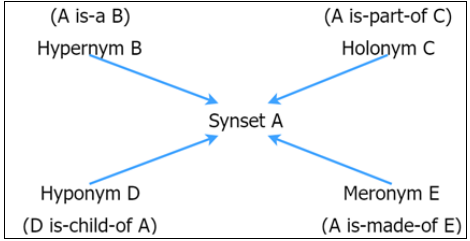
图1-2 同义词集各类关系图
1.2 利用NLTK中的WordNet进一步分析
首先,下载WordNet和wordnet corpus,如下
import nltk
nltk.download('wordnet')
from nltk.corpus import wordnet as wn
![]() 其次,查看同义词集各类关系
其次,查看同义词集各类关系
输入
# shows all the available synsets
word = 'car'
car_syns = wn.synsets(word)
print('All the available Synsets for ',word)
print('\t',car_syns,'\n')

# The definition of the first two synsets
syns_defs = [car_syns[i].definition() for i in range(len(car_syns))]
print('Example definitions of available Synsets ...')
for i in range(3):
    print('\t',car_syns[i].name(),': ',syns_defs[i])
print('\n')

# Get the lemmas for the first Synset
print('Example lemmas for the Synset ',car_syns[i].name())
car_lemmas = car_syns[0].lemmas()[:3]
print('\t',[lemma.name() for lemma in car_lemmas],'\n')

# Let us get hypernyms for a Synset (general superclass)
syn = car_syns[0]
print('Hypernyms of the Synset ',syn.name())
print('\t',syn.hypernyms()[0].name(),'\n')

# Let us get hyponyms for a Synset (specific subclass)
syn = car_syns[0]
print('Hyponyms of the Synset ',syn.name())
print('\t',[hypo.name() for hypo in syn.hyponyms()[:3]],'\n')

# Let us get part-holonyms for a Synset (specific subclass)
# also there is another holonym category called "substance-holonyms"
syn = car_syns[2]
print('Holonyms (Part) of the Synset ',syn.name())
print('\t',[holo.name() for holo in syn.part_holonyms()],'\n')

# Let us get meronyms for a Synset (specific subclass)
# also there is another meronym category called "substance-meronyms"
syn = car_syns[0]
print('Meronyms (Part) of the Synset ',syn.name())
print('\t',[mero.name() for mero in syn.part_meronyms()[:3]],'\n')
最后,看看词之间的相似度情况
word1, word2, word3 = 'car','lorry','tree'
w1_syns, w2_syns, w3_syns = wn.synsets(word1), wn.synsets(word2), wn.synsets(word3)

print('Word Similarity (%s)<->(%s): '%(word1,word2),wn.wup_similarity(w1_syns[0], w2_syns[0]))
print('Word Similarity (%s)<->(%s): '%(word1,word3),wn.wup_similarity(w1_syns[0], w3_syns[0]))
1.3 WordNet存在的不足
-
首先,细微差别体现不足。这是WordNet的一个重要不足。但这方面的不足有理论和实际两方面的原因。从理论的角度来看,对两个实体之间细微差别的定义进行建模是难以实现的。实际上,定义细微差别多数是主观的。例如,“想要”和“需要”两词有相似的含义,但其中“需要”更加肯定、更加坚定,这是一种细微差别。
-
其次,WordNet本身是主观的。因为WordNet是由一个相对较小的社区设计的。因此,取决于您试图解决的问题,WordNet可能是合适的,也可能有一个更好的方式去进行词定义。
-
WordNet维护成本高。这是劳动密集型的,维护和添加新的合成、定义、引理等,可能非常昂贵。
-
重新开发其他语言的WordNet成本昂贵。当然,也有一些努力来构建其他语言的WordNet,并将其与英文WordNet一起以MultiWordNet(MWN)形式出现,但还不完整。
2、独热编码(one-hot encoded)
其实,词表示的另一种更简单的方法就是one-hot-encoded,相关介绍已经很多,这里就举个例子来说明。如果我们有一V字型词汇表,对于每一个i对应的单词w i(i为w的下标),我们将用一个V长向量(0, 0, 0,…,0, 1, 0,…,0, 0, 0)表示单词w i,这里的第i个元素是1,其他元素全部是0。例如,以下面一句话为例,
Bob and Mary are good friends.
热编码每个单词的表示可能是这样的:
Bob: [1,0,0,0,0,0]
and: [0,1,0,0,0,0]
Mary: [0,0,1,0,0,0]
are: [0,0,0,1,0,0]
good: [0,0,0,0,1,0]
friends: [0,0,0,0,0,1]
在实际应用中,当你处理文本中的单词时,每一个单词可能需要从成百上千个类种进行预测出一个属于它的。而现在只有一个元素设置为1其余全部为0,显然,尝试对这些单词进行热编码是非常低效的。如图1-3所示,进入第一个隐藏层的矩阵乘法得到的值几乎全部为零,显然,这是一种巨大的计算浪费。

图1-3
另外,这种表示不以任何方式对单词之间的相似性进行编码,且完全忽略了使用词语所在的上下文语境。考虑到词向量之间的点积是相似性的度量:两个向量越相似,两个向量的点积越高;这种情况下,词’automobile‘和’car‘之间的相似度值为0,‘car’和‘hill’之间的相似度也是0,显然无法区分出两组单词间相似度的差异。
所以,这种方法对于大型词汇表来说是非常无效的。对于一个典型的NLP任务,词汇很容易超过50000个单词,因此,50000个词的词表示矩阵将导致非常稀疏的50000×50000矩阵。
但是,在最新的词嵌入学习算法中,one-hot encoed起到左右却不可忽视。我们使用一个热编码来表示数字化的词,并将其馈送到神经网络,使得神经网络可以学习更好和更小的数字化特征表示的单词。
3、TF-IDF
TF-IDF(Term Frequency-Inverse Document Frequency, 词频-逆文件频率)。是一种用于资讯检索与资讯探勘的常用加权技术。TF-IDF是一种统计方法,用以评估一字词对于一个文件集或一个语料库中的其中一份文件的重要程度。字词的重要性随着它在文件中出现的次数成正比增加,但同时会随着它在语料库中出现的频率成反比下降。一句话: 一个词语在一篇文章中出现次数越多, 同时在所有文档中出现次数越少, 越能够代表该文章.
词频 (term frequency, TF) 指的是某一个给定的词语在该文件中出现的次数。这个数字通常会被归一化(一般是词频除以文章总词数), 以防止它偏向长的文件。(同一个词语在长文件里可能会比短文件有更高的词频,而不管该词语重要与否。)但是, 需要注意, 一些通用的词语对于主题并没有太大的作用, 反倒是一些出现频率较少的词才能够表达文章的主题, 所以单纯使用是TF不合适的。权重的设计必须满足:一个词预测主题的能力越强,权重越大,反之,权重越小。所有统计的文章中,一些词只是在其中很少几篇文章中出现,那么这样的词对文章的主题的作用很大,这些词的权重应该设计的较大。IDF就是在完成这样的工作。
计算公式如下

举例说明,下面有两个文档
• Document 1: This is about cats. Cats are great companions.
• Document 2: This is about dogs. Dogs are very loyal.
直接套用公式计算:
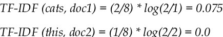
显然,“cats”这个词是带有有用信息的词,而“this”却不符合要求。在衡量词汇重要性或者说是特征选择时,TF-IDF方法是很重要的。
4、共生矩阵(Co-occurrence matrix)
共现矩阵不像独热编码对上下文语境下的单词进行编码,但却需要V×V的矩阵。举例说明,下面有两句话:
• Jerry and Mary are friends.
• Jerry buys flowers for Mary.
通过共现矩阵的方法,我们得到如下矩阵(因为矩阵是对称的,所以只显示矩阵的一个三角形状)。
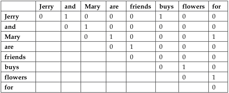
显然,不难看出,随着词汇规模的增加矩阵也随之迅速膨胀,维持共现矩阵需要的成本也随之急速扩大。此外,进行合并上下文窗口以便得到大于1的结果,也是比较困难的。如果进行加权计数,单词的权重也会随着相关词的距离增加而减少。
所有这些不足促使我们探索更具原则性、鲁棒性和可伸缩性的学习方式和推断词的意义(即表示)。Word2VEC是近期引入的分布式词表示学习技术,目前被用于许多NLP任务(例如机器翻译、聊天机器人和图像标题生成器)的特征工程技术。下面就重点探讨下Word2Vec--一种以神经网络为基础的方法去学习词表示。
四、Word2Vec
Word2vec,是为一群用来产生词向量的相关模型。这些模型为浅而双层的神经网络,用来训练以重新建构语言学之词文本。网络以词表现,并且需猜测相邻位置的输入词,在word2vec中词袋模型假设下,词的顺序是不重要的。训练完成之后,word2vec模型可用来映射每个词到一个向量,可用来表示词对词之间的关系,该向量为神经网络之隐藏层。
学习给定单词的意义,通过查看上下文并用数字表示。在上下文中,我们指的是在兴趣词前面和后面的固定数量的词。让我们假设一个有N个词的语料库。在数学上,这可以用W 0、W 1、…、W i和W n表示的单词序列来表示,其中w i是语料库中的第i个单词。
接下来,如果我们想找到一个能够学习单词意义的好算法,对于给定一个单词,我们的算法应该能够正确地预测上下文单词。这意味着对于任何给定的单词Wi,以下概率都是很高的:
为了得到等式右边部分,我们需要假定给定目标词(Wi)且上下文中词间是相互独立的(例如,Wi-1和Wi-2是独立的)。虽然不完全正确,但这种近似的取舍更加符合实际问题的解决。
1、Is queen = king -he + she ?(可以跳过)
这里和网上众多的“king”、‘man’、‘queen’、‘woman’都是类似的,之所以单独梳理下,是因为笔者在本书中发现了个问题,网上也没有发现合适的答案,记录下,以后有机会再回过头看看。
通过上面的资料,我们知道,为了更好地得到预期的词表示目标,需要最大化上面提到的概率,这里通过一个小的例子来进一步说明。下面这句话可以看做一个小的语料库。
There was a very rich king. He had a beautiful queen. She was very kind.
首先,人工做下预处理:删除标点符号和无信息的单词,结果如下:
was rich king he had beautiful queen she was kind
其次,对于每一个单词而言,我们给出多个元祖组合,上下文单词统一格式(目标词-->上下文单词1,上下文单词2)。假设在任一方的上下文窗口大小为1:
was → rich
rich → was, king
king → rich, he
he → king, had
had → he, beautiful
beautiful → had, queen
queen → beautiful, she
she → queen, was
was → she, kind
kind → was
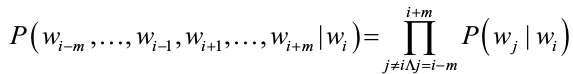
目标要清楚,那就是:在给出左边单词的情况下,我们能够预测右边的单词。为了实现这一点,右侧上下文的单词与左侧给定单词间应该拥有较高的相似度。也就是说,给定词义应该被其周围的词进一步传达。为了更好地理解,我们人为给出相关数值,以粗体单词为例。
rich → [0,0]
通过给定单词‘rich’,要准确地预测出‘was’和‘rich’,那么‘was’和‘king’与‘rich’之间应该有很高的相似度,这里以向量间欧几里得距离去衡量相似度。
下面给出‘king’和‘was’的数值,(英文原版中给出的单词‘rich’应该有误)
king → [0,1]
was → [-1,0]
我们很容易计算出相关欧氏距离,如下所示:
Dist(rich,king) = 1.0
Dist(rich,was) = 1.0
比较直观的欧式距离表示如图4-1所示:
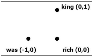
图4-1
同样,我们继续下面单词元组间的梳理:
king → rich, he
我们已经建立了‘king'和’rich‘间的关系,但相关工作还没有完成;下一步先调整’king‘的矢量,使之更接近于’rich‘:
king → [0,0.8]
接下来,我们把单词’he‘添加到图示中,’he‘应该更接近’king‘,这就是目前为关于右边‘he’单词的所有信息。
he → [0.5,0.8]
此时,图示如4-2所示:
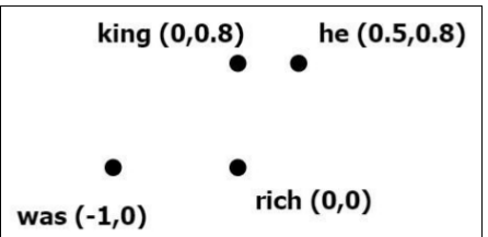
图4-2
继续下面两个元组:queen-->beautiful,she 和she-->queen,was。
she → queen, was
现在,我们用对英语的先验知识来进一步研究。由于‘she’和‘he’在上下文中的用法是等价的或者是等概率的,所以‘she‘到’was‘和’he‘到’was‘之间的距离是等同的,则:
she → [0.5,0.6]
备注:存在的问题,那就是既然’she‘到’was‘和’he‘到的距离是相等的,那么直接在下面二维图示中显示was(-1,0),he(0.5,0.8),she(0.5,0.6)显示是有问题的。笔者也查看了网上的文章,目前为止没有找到讲解这个问题的文章,常见的说法是“一些研究还发现,计算有相似关系的单词之间的位移向量也会十分相似,例如从‘Man’到‘Wonman’的向量,与从‘King’到‘Queen’之间的向量几乎相同”,来对Word2Vec进行解释,具体验证没发现。如果有网友清楚这一块的,请帮忙解释一下。这里暂且按常识性的来开展。
下一步,用“queen”接近“she”:
queen → [0.0,0.6]
最终形成如图4-3所示:
图4-3
截止目前,显然方程的右边和左边是相等的:
右边= king – he + she
= [0,0.8] – [0.5,0.8] + [0.5,0.6]
= [0,0.6]
左边=[0,0.6]
即 queen = king -he + she。
2、设计学习词嵌入的损失函数
现实世界中,即使是一个比较简单任务,其单词量也很容易超过10000个,因此,对于开发大型文本语料库中单词向量的艰巨任务,靠 人工去完成显然是不合适,我们可以设计一种方法,比如使用一些 机器学习算法(例如神经网络等)自动找到合适的词嵌入。对于使用机器学习算法来完成任务而言,需要定义一个损失函数,使其损失最小化。

接着定义一个神经网络代价(损失)函数
这里需要对 
下面我们将方程转换为日志空间,前后的一致性和数值稳定性会更佳,如下:
上面这个公式就是众所周知的负对数似然。
现在我们得到了一个代价函数,就可以使用神经网络来优化这个代价函数,这样会使得词向量或词嵌入根据词的意思更好地组合自身。
3、Skip-Gram模型
3.1 简要说明
对于Word2Vec而言,其模型主要有Skip-Gram和CBOW两种,简单来讲,已知一个单词Wt,去实现预测其前后W(t-2)、W(t-1)、W(t+1)、W(t+2)上下文词的方法,就是Skip-Gram方法;而反过来,给出W(t-2)、W(t-1)、W(t+1)、W(t+2)单词,去预测Wt的方法,就是CBOW方法。
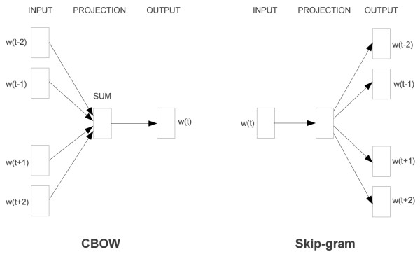
图4-4
Skip-Gram模型的搭建包括两个部分:一是建立模型,二是通过模型获取嵌入词向量。Skip-Gram建模思想与自编码器(auto-encoder)很相似,都是先基于训练数据建立一个神经网络,当这个模型训练好以后,我们得到该模型训练过程中所学到的参数,常见的有隐藏层的权重矩阵等,显然这只是我们实现目标过程中必要的铺垫工作,所以,有文章也称基于训练数据建模的过程为“Fake Task”。
3.2 The Fake Task
在上面提到,训练模型目的是为了获得模型基于训练数据学到的隐藏层权重。为了获得这些权重,我们首先要建立一个完整的神经网络作为“Fake Task”,后续再回头来看通过“Fake Task”如何间接地得到这些词向量。举例说明,这里有一个句子“The dog barked at the mailman”。
-
首先我们选句子中间的一个词作为我们的输入词,例如我们选取“dog”作为input word;
-
有了input word以后,我们再定义一个叫做skip_window的参数,它代表着我们从当前input word的一侧(左边或右边)选取词的数量。如果我们设置skip_window=2,那么我们最终获得窗口中的词(包括input word在内)就是['The', 'dog','barked', 'at']。skip_window=2代表着选取左input word左侧2个词和右侧2个词进入我们的窗口,所以整个窗口大小span=2x2=4。另一个参数叫num_skips,它代表着我们从整个窗口中选取多少个不同的词作为我们的output word,当skip_window=2,num_skips=2时,我们将会得到两组 (input word, output word) 形式的训练数据,即 ('dog', 'barked'),('dog', 'the')。
-
神经网络基于这些训练数据将会输出一个概率分布,这个概率代表着词典中的每个词是output word的可能性。结合例子说明,上一步中我们在设置skip_window和num_skips=2的条件下获得了两组训练数据。若先拿一组数据 ('dog', 'barked') 来训练神经网络,那么模型通过学习这个训练样本,会告诉我们词汇表中每个单词是“barked”的概率大小。
模型的输出概率代表着词典中每个词有多大概率与input word同时出现。例如,如果向神经网络模型中输入一个单词“Chinese“,那么最终模型的输出概率中,像“China”, “Confucius”这种相关词的概率将远高于像”watermelon“,”kangaroo“非相关词的概率。因为”China“,“Confucius”在文本中更大可能在”Chinese“的窗口中出现。我们将通过给神经网络输入文本中成对的单词来训练它完成上面所说的概率计算。下面的图中给出了一些训练样本的例子。这里选定句子“The quick brown fox jumps over lazy dog”,设定我们的窗口大小为2(window_size=2),即仅选输入词前后各两个词和输入词进行组合。图4-5中,蓝色代表input word,方框内代表位于窗口内的单词。
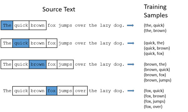
图4-5
这里的模型将会从每对单词出现的次数中习得统计结果。例如,神经网络可能会得到更多类似(“Chinese“,”China“)这样的训练样本对,而对于(”Chinese“,”watermelon“)这样的组合却看到的很少。因此,当模型完成训练后,给定一个单词”Chinese“作为输入,输出的结果中”Chinese“或者”Confucius“要比”watermelon“被赋予更高的概率。
3.3 模型结构分析
上面曾提到,通过机器学习算法来开展任务的话,所有输入值必须被数字化。这里,将基于训练文档来构建我们自己的词汇表(vocabulary)后,再对单词进行独热编码(one-hot编码)。
假定从训练文档中抽取10000个唯一不重复的单词组成词汇表。对这些10000个单词进行独热编码(one-hot编码),得到的每个单词都是一个10000维的向量,向量每个维度的值只有0或者1,假如单词ants在词汇表中的出现位置为第3个,那么ants的向量就是一个第三维度取值为1,其他维都为0的10000维的向量(ants=[0, 0, 1, 0, ..., 0])。
对于“The dog barked at the mailman”而言,基于这个句子,可以构建一个大小为5的词汇表(大小写和标点符号不需要,可以忽略):("the", "dog", "barked", "at", "mailman"),我们对这个词汇表的单词进行编号0-4。那么”dog“就可以被表示为一个5维向量[0, 1, 0, 0, 0]。
模型的输入如果是一个10000维的向量,那么输出也应是一个10000维度(词汇表的大小)的向量,它包含了10000个概率,每一个概率代表着当前词是输入样本中output word的概率大小。
图4-6是神经网络的结构:

![]()
图4-6
在隐藏层没有使用任何激活函数,但是在输出层使用了sotfmax函数。
通过成对的单词来对神经网络进行训练,训练样本是 ( input word, output word ) 这样的词对,input word和output word都是one-hot编码的向量。最终模型的输出是一个概率分布。
3.4 隐藏层
单词的编码和训练样本选取之后,下面说下隐层。假设现在用300个特征来表示一个单词(即每个词被表示为300维的向量),那么隐藏层的权重矩阵应该表示为10000行、300列(隐藏层有300个结点)。
词向量的维度是一个可以调节的超参数,Python开发里的gensim包中封装的Word2Vec接口默认词向量大小为100, window_size为5。
图4-7中左右两张子图分别给出了不同角度下输入层-隐层的权重矩阵表示形式。左图中每一列代表一个10000维的词向量和隐层单个神经元连接的权重向量。右的图中每一行实际上代表了每个单词的词向量。
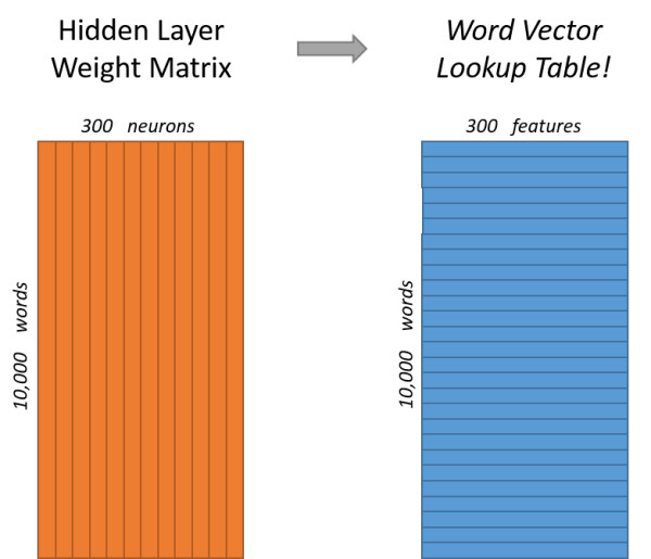
图4-7
综合来看,这里的目标是学习这个隐层的权重矩阵。现在 继续通过模型的定义来训练这个模型。
上面我们提到,通过one-hot encoded对input word和output word编码。进一步查看可知,最初的输入被one-hot编码以后,除了一个位置为1其余维度全部是0,所以这个向量相当稀疏,会产生很多没必要的计算成本,多数计算是无效的。例如,将一个1 x 10000的向量和10000 x 300的矩阵相乘,它会消耗相当大的计算资源。显然,为了高效计算,选择矩阵中对应的向量中维度值为1的索引行是个明智的选择,就像图4-8所示
![]()
![]()
图4-8
上图中的矩阵运算,左边分别是1 x 5和5 x 3的矩阵,结果应该是1 x 3的矩阵,按照矩阵乘法的规则,结果的第一行第一列元素为0 x 17 + 0 x 23 + 0 x 4 + 1 x 10 + 0 x 11 = 10,同理可得其余两个元素为12,19。如果10000个维度的矩阵采用这样的计算方式是十分低效的。
为了高效地利用计算资源,这种稀疏状态下不会进行矩阵乘法计算,最优矩阵的计算的结果实际上是矩阵对应向量中值为1的索引。这里,左边向量中取值为1的对应的维度为3(下标从0开始),则计算结果就是矩阵的第3行(下标从0开始)—— [10, 12, 19],这样模型中的隐层权重矩阵便成了一个”查找表“(lookup table),进行矩阵计算时,直接去查输入向量中取值为1的维度下对应的那些权重值。隐藏层的输出就是每个输入单词的“嵌入词向量”。
3.5 输出层
经过神经网络隐层的计算,ants这个词会从一个1 x 10000的向量变成1 x 300的向量,再被输入到输出层。输出层是一个softmax回归分类器,它的每个结点将会输出一个0-1之间的值(概率),这些所有输出层神经元结点的概率之和为1。
图4-9是一个例子,训练样本为 (input word: “ants”, output word: “car”) 的计算示意图。

图4-9
3.6 利用Tensorflow来开展Skip-gram模型
这里分别给出Skip-gram模型的概念和实施层面的大致思路图。图4-10相关说明、图4-11 是概念框架、图4-12是实施框架明,
图4-10
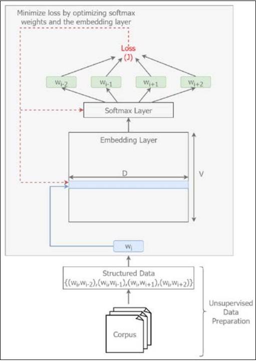
图4-11 Skip-gram概念模型
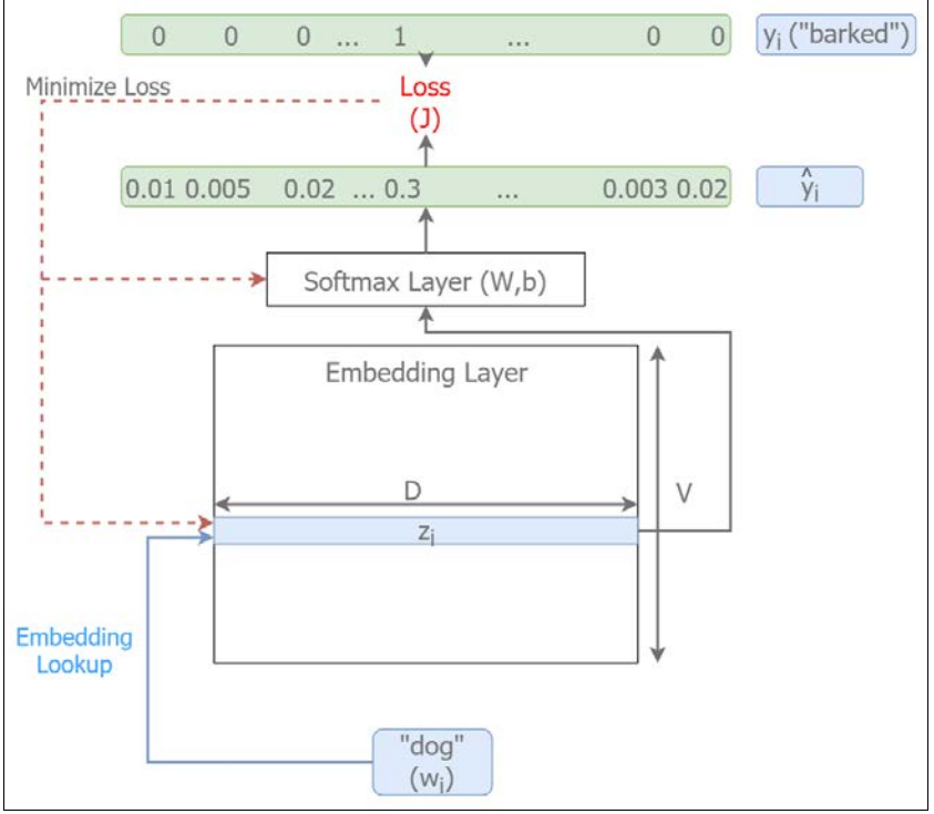
图4-12 Skip-gram实施模型
3.6.1 数据集
这里采用由几个维基百科文章组成的数据集,下载地址 Data。限于篇幅,这里给出关键代码部分。
代码如下
url = 'http://www.evanjones.ca/software/'

def maybe_download(filename, expected_bytes):
  """Download a file if not present, and make sure it's the right size."""
  if not os.path.exists(filename):
    print('Downloading file...')
    filename, _ = urlretrieve(url + filename, filename)
  statinfo = os.stat(filename)
  if statinfo.st_size == expected_bytes:
    print('Found and verified %s' % filename)
  else:
    print(statinfo.st_size)
    raise Exception(
      'Failed to verify ' + filename + '. Can you get to it with a browser?')
  return filename

filename = maybe_download('wikipedia2text-extracted.txt.bz2', 18377035)
![]()
3.6.2 相关步骤
-
用NLTK对数据进行预处理;
-
建立相关Dictionaries,包括word到ID、ID到word及单词list(word,frequency)等;
-
给出数据的Batches;
-
明确超参数、输出样本、输入样本、参数及其他变量;
-
计算单词相似性;
-
模型优化、执行;
-
利用 t-SNE Results给出可视化结果;
考虑篇幅问题,这里给出产生数据Batches和模型运行的代码。
1)、Generating Batches of Data for Skip-Gram
data_index = 0

def generate_batch_skip_gram(batch_size, window_size):
  # data_index is updated by 1 everytime we read a data point
  global data_index

  # two numpy arras to hold target words (batch)
  # and context words (labels)
  batch = np.ndarray(shape=(batch_size), dtype=np.int32)
  labels = np.ndarray(shape=(batch_size, 1), dtype=np.int32)

  # span defines the total window size, where
  # data we consider at an instance looks as follows.
  # [ skip_window target skip_window ]
  span = 2 * window_size + 1

  # The buffer holds the data contained within the span
  buffer = collections.deque(maxlen=span)

  # Fill the buffer and update the data_index
  for _ in range(span):
    buffer.append(data[data_index])
    data_index = (data_index + 1) % len(data)

  # This is the number of context words we sample for a single target word
  num_samples = 2*window_size

  # We break the batch reading into two for loops
  # The inner for loop fills in the batch and labels with
  # num_samples data points using data contained withing the span
  # The outper for loop repeat this for batch_size//num_samples times
  # to produce a full batch
  for i in range(batch_size // num_samples):
    k=0
    # avoid the target word itself as a prediction
    # fill in batch and label numpy arrays
    for j in list(range(window_size))+list(range(window_size+1,2*window_size+1)):
      batch[i * num_samples + k] = buffer[window_size]
      labels[i * num_samples + k, 0] = buffer[j]
      k += 1

    # Everytime we read num_samples data points,
    # we have created the maximum number of datapoints possible
    # withing a single span, so we need to move the span by 1
    # to create a fresh new span
    buffer.append(data[data_index])
    data_index = (data_index + 1) % len(data)
  return batch, labels

print('data:', [reverse_dictionary[di] for di in data[:8]])

for window_size in [1, 2]:
    data_index = 0
    batch, labels = generate_batch_skip_gram(batch_size=8, window_size=window_size)
    print('\nwith window_size = %d:' %window_size)
    print('    batch:', [reverse_dictionary[bi] for bi in batch])
    print('    labels:', [reverse_dictionary[li] for li in labels.reshape(8)])
相应输出为
data: ['propaganda', 'is', 'a', 'concerted', 'set', 'of', 'messages', 'aimed']
with window_size = 1:
    batch: ['is', 'is', 'a', 'a', 'concerted', 'concerted', 'set', 'set']
    labels: ['propaganda', 'a', 'is', 'concerted', 'a', 'set', 'concerted', 'of']
with window_size = 2:
    batch: ['a', 'a', 'a', 'a', 'concerted', 'concerted', 'concerted', 'concerted']
    labels: ['propaganda', 'is', 'concerted', 'set', 'is', 'a', 'set', 'of']
2)、Running the Skip-Gram Algorithm
num_steps = 100001
skip_losses = []
# ConfigProto is a way of providing various configuration settings
# required to execute the graph
with tf.Session(config=tf.ConfigProto(allow_soft_placement=True)) as session:
  # Initialize the variables in the graph
  tf.global_variables_initializer().run()
  print('Initialized')
  average_loss = 0

  # Train the Word2vec model for num_step iterations
  for step in range(num_steps):

    # Generate a single batch of data
    batch_data, batch_labels = generate_batch_skip_gram(
      batch_size, window_size)

    # Populate the feed_dict and run the optimizer (minimize loss)
    # and compute the loss
    feed_dict = {train_dataset : batch_data, train_labels : batch_labels}
    _, l = session.run([optimizer, loss], feed_dict=feed_dict)

    # Update the average loss variable
    average_loss += l

    if (step+1) % 2000 == 0:
      if step > 0:
        average_loss = average_loss / 2000

      skip_losses.append(average_loss)
      # The average loss is an estimate of the loss over the last 2000 batches.
      print('Average loss at step %d: %f' % (step+1, average_loss))
      average_loss = 0

    # Evaluating validation set word similarities
    if (step+1) % 10000 == 0:
      sim = similarity.eval()
      # Here we compute the top_k closest words for a given validation word
      # in terms of the cosine distance
      # We do this for all the words in the validation set
      # Note: This is an expensive step
      for i in range(valid_size):
        valid_word = reverse_dictionary[valid_examples[i]]
        top_k = 8 # number of nearest neighbors
        nearest = (-sim[i, :]).argsort()[1:top_k+1]
        log = 'Nearest to %s:' % valid_word
        for k in range(top_k):
          close_word = reverse_dictionary[nearest[k]]
          log = '%s %s,' % (log, close_word)
        print(log)
  skip_gram_final_embeddings = normalized_embeddings.eval()

# We will save the word vectors learned and the loss over time
# as this information is required later for comparisons
np.save('skip_embeddings',skip_gram_final_embeddings)

with open('skip_losses.csv', 'wt') as f:
    writer = csv.writer(f, delimiter=',')
    writer.writerow(skip_losses)
![]()
相关输出为(内容太多,给出中间部分没有罗列)
Initialized
Average loss at step 2000: 3.991611
Average loss at step 4000: 3.627553
Average loss at step 6000: 3.583732
Average loss at step 8000: 3.513987
Average loss at step 10000: 3.492103
Nearest to his: indifferentism, amnesty, ethnographic, sheesh, banking, scot, bran, chamillionaire,
Nearest to a: the, manchukuo, an, archipelagos, deaf, fins, communion, —,
Nearest to it: this, outlying, not, 296, goats, messenger, reconstruct, socialized,
Nearest to from: 1933., of, rap, dietitians, and, blanc, agraristas, technicians,

Nearest to not: so, although, it, if, but, also, they, even,
Nearest to to: sania, prank, would, with, will, place-names, for, subpixels,
Nearest to has: had, have, since, is, devín, marcel, was, dcen,
Nearest to .: ,, ;, that, and, the, dhexe, of, vain,
Nearest to of: for, in, ,, ., and, with, 's, victors,
Nearest to :: ;, newest, ``, three, include, wiesenthal, rexroth, entanglement,
Nearest to be: have, billed, welles, pleas, crusaders, preordered, persevered, are,
Average loss at step 92000: 3.298772
Average loss at step 94000: 3.252265
Average loss at step 96000: 3.286938
Average loss at step 98000: 3.288883
Average loss at step 100000: 3.275468
Nearest to his: their, 's, work, he, david, her, its, him,
Nearest to a: the, an, 's, this, first, spiders, another, pontus,
Nearest to it: she, not, he, that, this, said, also, what,
Nearest to from: between, in, calvin, during, about, over, up, 1587,
Nearest to at: on, counterrevolutionaries, year, after, debacle, malayo-polynesian, broadcast, for,
Nearest to 's: the, first, and, a, of, his, was, another,
Nearest to with: between, after, while, and, like, from, rascia, qualities,
Nearest to ,: ., and, in, of, the, on, ', to,
Nearest to this: also, another, it, an, the, a, sinicized, vested,
Nearest to not: it, still, so, n't, also, they, that, although,
Nearest to to: would, ,, and, matched, of, will, could, uninteresting,
Nearest to has: have, had, was, is, since, fifty, arterial, albrecht,
Nearest to .: ,, ;, and, ', jefferson, that, ``, of,
Nearest to of: ,, in, and, 's, on, album, the, .,
Nearest to :: ;, three, two, nematode, one, (, '', ],
Nearest to be: have, him, hunua, categorise, hear, billed, sedimentary, tee-shirts,
3)、通过t-SNE给出的可视化结果如图4-13所示
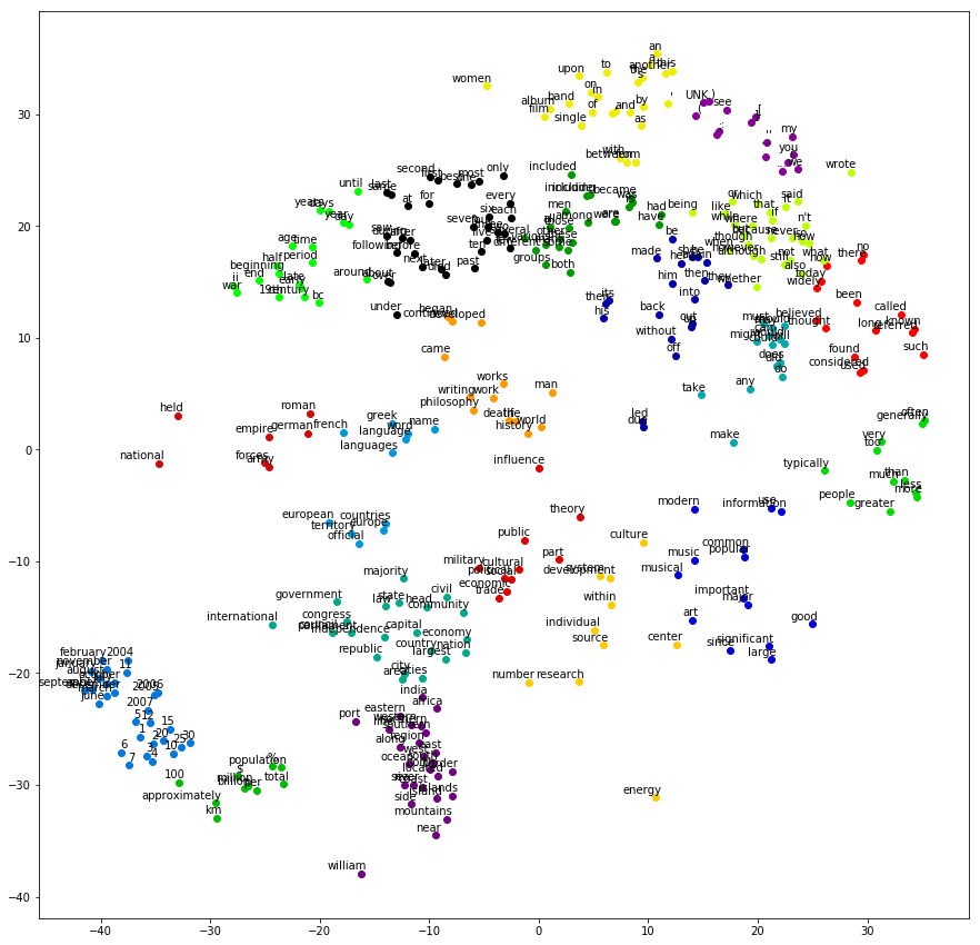
图4-13
4、 CBOW(Continuous Bag-of-Words)模型
4.1 简要概述
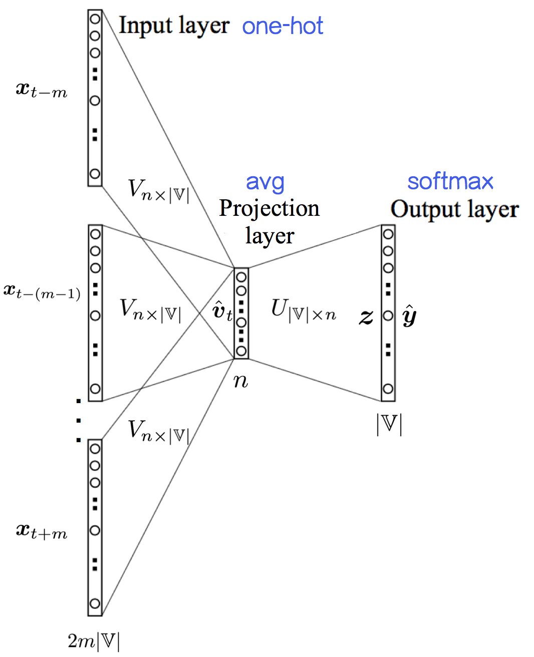
不带加速的CBOW模型是一个两层结构,相比于NPLM来说CBOW模型没有隐层,通过上下文来预测中心词,并且抛弃了词序信息——
输入层:n个节点,上下文共 2m 个词的词向量的平均值;
输入层到输出层的连接边:输出词矩阵 ![]() ;
;

输出层:|𝕍|个节点。第 i 个节点代表中心词是词 ![]() 的概率。
的概率。

如果要视作三层结构的话,可以认为——
输入层:2m×|𝕍|个节点,上下文共 2m 个词的one-hot representation
输入层到投影层到连接边:输入词矩阵 ![]() ;
;

投影层::n个节点,上下文共 2m 个词的词向量的平均值;
投影层到输出层的连接边:输出词矩阵![]() ;
;
输出层:|𝕍| 个节点。第 i 个节点代表中心词是词![]() 的概率。
的概率。
这样表述相对清楚,将one-hot到word embedding那一步描述了出来。这里的投影层并没有做任何的非线性激活操作,直接就是Softmax层。换句话说,如果只看投影层到输出层的话,其实就是个Softmax回归模型,但标记信息是词串中心词,而不是外部标注。见图4-14
![]()
图4-14
4.2 Softmax
不存在隐藏层的情况下,处理大型语料库计算量是相当大的,这里的解决方法也是通常用的的降维操作,即层次Softmax简化操作。以1000万的语料库来说,只选取我们需要的那些重要的单词。这里使用层次的Softmax操作。
在机器学习中,对要输出特征在预测结果中的重要性,选择树模型较多,因为树在节点选择分裂时,就是选择了包含信息量大的特征进行分裂,在这里的原理也一样。见图4-15

图4-15
也就是,在节点处的词出现的频数比较多、比较重要的词,换句话讲,在构建树时能体现这样频次的差别。
最典型的是使用赫夫曼树(Huffman Tree)来编码输出层的词典,赫夫曼树的的想法也很简单,就是对每个词根据频次有个权重,然后根据两颗子树进行拼接,最后离根节点越近的词,其出现的频率会更高,而在叶子节点处出现的频率更低。
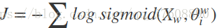
原来计算的是一个1000万的概率向量,现在则可以转换为一个二分类问题,二分类中最简单直接的是LR模型。假设![]()

就是一个词向量表示,在每个非叶子节点处(图中黄色的圆点)还会有一个参数![]()

,那我们的在LR中可以用一个sigmoid函数来映射,最后可以变成一个最小化损失函数
![]()
4.3 负例采样
负例采样操作起来简单粗暴,这里不做过多解读,网上有不少相关文章。这里值给出负例采样流程图,见图4-16.
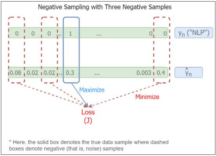
图4-16
4.4 CBOW模型图示
模型图示如图4-17

图4-17
4.5 CBOW模型的Tensorflow过程
4.5.1 相关流程如下:
-
沿用Skip-gram模型使用的样本;
-
建立一个新的数据 generator;
-
定义超参数、输出样本、输入样本、参数及其他变量;
-
计算单词相似性;
-
模型优化、执行;
-
利用 t-SNE Results给出可视化结果;
这里给出新建数据Grenerator和CBOW模型执行核心代码。
4.5.2 建立一个新的数据 generator
data_index = 0

def generate_batch_cbow(batch_size, window_size):
    # window_size is the amount of words we're looking at from each side of a given word
    # creates a single batch

    # data_index is updated by 1 everytime we read a set of data point
    global data_index

    # span defines the total window size, where
    # data we consider at an instance looks as follows.
    # [ skip_window target skip_window ]
    # e.g if skip_window = 2 then span = 5
    span = 2 * window_size + 1 # [ skip_window target skip_window ]

    # two numpy arras to hold target words (batch)
    # and context words (labels)
    # Note that batch has span-1=2*window_size columns
    batch = np.ndarray(shape=(batch_size,span-1), dtype=np.int32)
    labels = np.ndarray(shape=(batch_size, 1), dtype=np.int32)

    # The buffer holds the data contained within the span
    buffer = collections.deque(maxlen=span)

    # Fill the buffer and update the data_index
    for _ in range(span):
        buffer.append(data[data_index])
        data_index = (data_index + 1) % len(data)

    # Here we do the batch reading
    # We iterate through each batch index
    # For each batch index, we iterate through span elements
    # to fill in the columns of batch array
    for i in range(batch_size):
        target = window_size  # target label at the center of the buffer
        target_to_avoid = [ window_size ] # we only need to know the words around a given word, not the word itself

        # add selected target to avoid_list for next time
        col_idx = 0
        for j in range(span):
            # ignore the target word when creating the batch
            if j==span//2:
                continue
            batch[i,col_idx] = buffer[j]
            col_idx += 1
        labels[i, 0] = buffer[target]

        # Everytime we read a data point,
        # we need to move the span by 1
        # to create a fresh new span
        buffer.append(data[data_index])
        data_index = (data_index + 1) % len(data)

    return batch, labels

for window_size in [1,2]:
    data_index = 0
    batch, labels = generate_batch_cbow(batch_size=8, window_size=window_size)
    print('\nwith window_size = %d:' % (window_size))
    print('    batch:', [[reverse_dictionary[bii] for bii in bi] for bi in batch])
    print('    labels:', [reverse_dictionary[li] for li in labels.reshape(8)])
输出为
with window_size = 1:
    batch: [['propaganda', 'a'], ['is', 'concerted'], ['a', 'set'], ['concerted', 'of'], ['set', 'messages'], ['of', 'aimed'], ['messages', 'at'], ['aimed', 'influencing']]
    labels: ['is', 'a', 'concerted', 'set', 'of', 'messages', 'aimed', 'at']

with window_size = 2:
    batch: [['propaganda', 'is', 'concerted', 'set'], ['is', 'a', 'set', 'of'], ['a', 'concerted', 'of', 'messages'], ['concerted', 'set', 'messages', 'aimed'], ['set', 'of', 'aimed', 'at'], ['of', 'messages', 'at', 'influencing'], ['messages', 'aimed', 'influencing', 'the'], ['aimed', 'at', 'the', 'opinions']]
    labels: ['a', 'concerted', 'set', 'of', 'messages', 'aimed', 'at', 'influencing']
4.5.3 CBOW模型执行
num_steps = 100001
cbow_losses = []

# ConfigProto is a way of providing various configuration settings
# required to execute the graph
with tf.Session(config=tf.ConfigProto(allow_soft_placement=True)) as session:

    # Initialize the variables in the graph
    tf.global_variables_initializer().run()
    print('Initialized')

    average_loss = 0

    # Train the Word2vec model for num_step iterations
    for step in range(num_steps):

        # Generate a single batch of data
        batch_data, batch_labels = generate_batch_cbow(batch_size, window_size)

        # Populate the feed_dict and run the optimizer (minimize loss)
        # and compute the loss
        feed_dict = {train_dataset : batch_data, train_labels : batch_labels}
        _, l = session.run([optimizer, loss], feed_dict=feed_dict)

        # Update the average loss variable
        average_loss += l

        if (step+1) % 2000 == 0:
            if step > 0:
                average_loss = average_loss / 2000
                # The average loss is an estimate of the loss over the last 2000 batches.
            cbow_losses.append(average_loss)
            print('Average loss at step %d: %f' % (step+1, average_loss))
            average_loss = 0

        # Evaluating validation set word similarities
        if (step+1) % 10000 == 0:
            sim = similarity.eval()
            # Here we compute the top_k closest words for a given validation word
            # in terms of the cosine distance
            # We do this for all the words in the validation set
            # Note: This is an expensive step
            for i in range(valid_size):
                valid_word = reverse_dictionary[valid_examples[i]]
                top_k = 8 # number of nearest neighbors
                nearest = (-sim[i, :]).argsort()[1:top_k+1]
                log = 'Nearest to %s:' % valid_word
                for k in range(top_k):
                    close_word = reverse_dictionary[nearest[k]]
                    log = '%s %s,' % (log, close_word)
                print(log)
    cbow_final_embeddings = normalized_embeddings.eval()


np.save('cbow_embeddings',cbow_final_embeddings)

with open('cbow_losses.csv', 'wt') as f:
    writer = csv.writer(f, delimiter=',')
    writer.writerow(cbow_losses)
![]()
输出部分(内容多,给出部分输出结果)
Initialized
Average loss at step 2000: 3.571350
Average loss at step 4000: 3.077189
Average loss at step 6000: 2.951976
Average loss at step 8000: 2.868055
Average loss at step 10000: 2.796585
Nearest to with: nederlandse, abbr, canaan, ars, brochure, ester, comte, rubberized,
Nearest to other: nuclear, 1419, restore, some, teammates, unrepresented, mothe, both,
Nearest to '': hungarorum, paws, }, updrafts, hatta, dementing, ca, titled,
Nearest to to: schmitz, norwood, would, bleak, 1855., arsonists, inferring, athletics,
Nearest to on: ascendancy, dynamo, mcqueen, guyana, csc, on-die, tennessee, a.f.c.,
ssicism, mimesis, resting, actually,
Nearest to had: have, has, having, carboxylic, remained, dunkirk, leikin, checker,
Nearest to ;: ., ,, —, expressionistic, conch, commutes, furry, venation,
Average loss at step 92000: 2.102314
Average loss at step 94000: 2.097561
Average loss at step 96000: 2.110340
Average loss at step 98000: 2.095927
Average loss at step 100000: 2.108117
Nearest to with: toxteth, 21., 102,800, dubuque, mid-to-late, vernal, validate, abbr,
Nearest to other: woolshed, various, top-loading, pia, dye, these, zwan, teammates,
Nearest to '': divining, titled, subfreezing, dementing, война, word, neubrandenburg, hiphop,
Nearest to to: bleak, might, schmitz, helped, towards, norwood, will, must,
Nearest to on: upon, ascendancy, 27th, csc, rotherhithe, feces, cheer, muskogee,
Nearest to ): e.g, orléans, mazzola, driving, metres, nightfall, 687., 2,341,
Nearest to his: her, their, my, its, osiris, xor, intestines, digitally,
Nearest to this: it, 98.6, similar, citation, tyresö, budgetary, marge, these,
Nearest to one: glens, enforcing, recovered, 400-series, claudius, rejoin, surviving, smiling,
Nearest to which: where, but, whom, whose, −50, stolen, moneda, polarization,
Nearest to not: n't, rarely, never, vegetative, still, opt, sardis, spouses,
Nearest to but: however, though, which, although, especially, whereas, including, footprints,
Nearest to were: are, lech, was, sintering, been, re-evaluation, unclassified, symbolizing,
Nearest to also: now, still, billionaires, cleveland, neo-classicism, resting, ductile, zemin,
Nearest to had: having, has, have, dunkirk, downplayed, carboxylic, hancock, remained,
Nearest to ;: ., ,, —, conch, expressionistic, :, commutes, storing,
词嵌入已经成为许多NLP任务中的重要组成部分,并且被广泛地应用于诸如机器翻译、聊天机器人、图像标题生成和语言建模等任务。词嵌入不仅是一种降维技术(与one-hot encoded相比),而且也在特征表示方面比其他技术更加实用。本文重点讨论了基于神经网络的两种学习词表示的方法,即Skip-gram模型和CBOW模型。
首先,我们讨论了一些传统方法,对于词表示或者词意义有了更多的理解。在这个过程中,我们实用了WordNet、建立了一些单词的共现矩阵、计算了TF-IDF值,并讨论了这些传统方法的局限性。
传统方法的局限性,促使我们继续探索基于神经网络的词表示学习方法。qingk
最后,我们重点讨论了损失函数、Skip-gram模型和CBOW模型各自原理情况,并通过Tensorflow方法一一做了模型实施,给出了最后的输出结果,让我们对于两个模型有更加深入的理解。下一步将重点探讨下SKip-gram、CBOW比较及著名的Global Vectors (GloVe)模型。
主要参考资料 《Natural Language Processing with TensorFlow》(Thushan Ganegedara; 2018 Packt Publishing;First published: May 2018)
部分参考资料

 浙公网安备 33010602011771号