
< - OPENGL 13 PBR - >
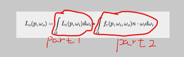
PBR Opengl 的应用,理想,完美的公式,这公式在BRDF不知道的情况下完全废物:
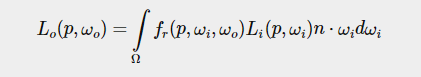
所以现在引入一个最简单的BRDF模型:Cook-Torrance BRDF:

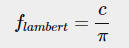
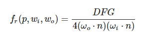
左边是lambertian部分,右边是高光部分。能量守恒部分肯定要满足 diffuse部分+镜面部分 <=1

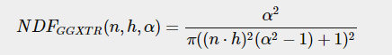
公式中DFG全部为一个函数。或者由几个函数组成。
D:Normal distribution function,h是half vertor, a其实是roughness,这个公式称作Trowbridge-Reitz GGX:
一般代码表示这个D的返回值都是ggx_tr(),输入3个参数,法线,半向量,roughness
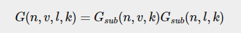
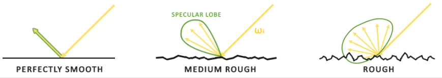
G:Geometry function,经过实际测试,就是灯光照亮微平面的遮蔽效果。类似阴影,但是又不是阴影。
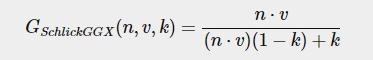
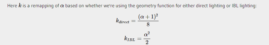
其中k比较特殊,在IBL中和灯光直接照明意义不一样。
正确的G还要考虑灯光向量进去。所以Smith's method:
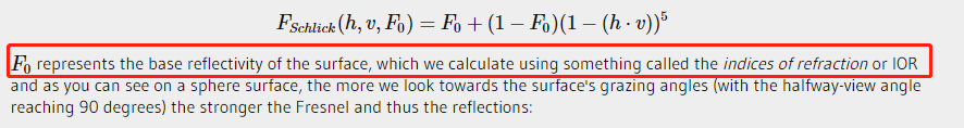
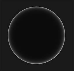
F: 菲尼尔方程用Fresnel-Schlick近似法:F0 是indices of refraction or IOR
合并到一块:
分开积分相加:
可以看到分为Kd(diffuse部分) Ks(specular reflection部分)。
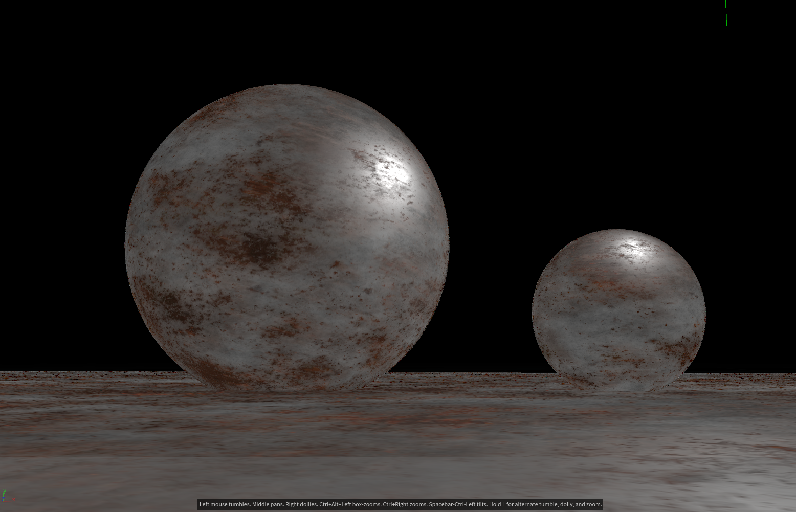
开局给你一个球:DEBUG In houdini
1,一般灯光GGX VIS:


vector lgtpos = chv("lgtpos");
float rough = chf("rough");
vector wi = normalize(lgtpos - @P);
vector wo = normalize(campos - @P);
vector h = normalize(wi+wo);

float lambert = max(dot(@N, wi), 0);


float D_GGX_TR(vector N;vector H;float a)
{
    float a2     = a*a;
    float NdotH  = max(dot(N, H), 0.0);
    float NdotH2 = NdotH*NdotH;

    float nom    = a2;
    float denom  = (NdotH2 * (a2 - 1.0) + 1.0);
    denom        = PI * denom * denom;

    return nom / denom;
}

vector rough_tex = texture(chs("image"),@uv.x, @uv.y);
vector diff = texture(chs("diff"),@uv.x, @uv.y);


float ggx = D_GGX_TR(@N,h,rough_tex.x );


@Cd = diff  + ggx*0.5 ;
Roughness:0.106
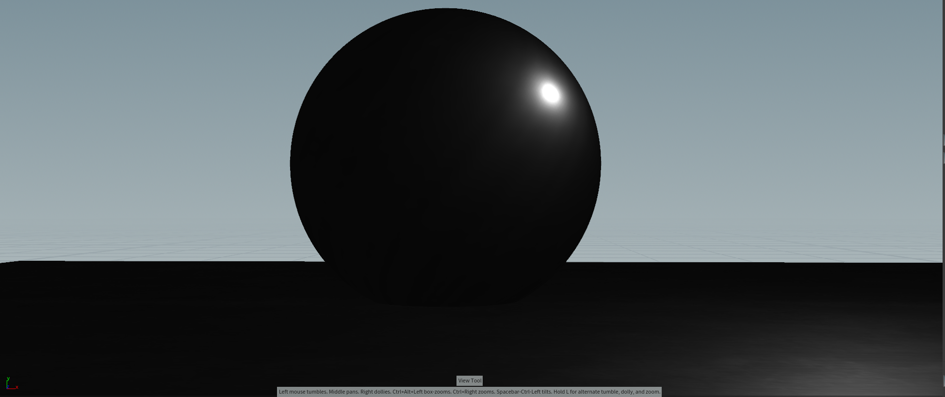
Roughness:0.315

完全给你一个球:
Normal distribution function + geometry function
vector campos = chv("campos");
vector lgtpos = chv("lgtpos");
float rough = chf("rough");
vector wi = normalize(lgtpos - @P);
vector wo = normalize(campos - @P);
vector h = normalize(wi+wo);

float lambert = max(dot(@N, wi), 0);


float D_GGX_TR(vector N;vector H;float a)
{
    float a2     = a*a;
    float NdotH  = max(dot(N, H), 0.0);
    float NdotH2 = NdotH*NdotH;

    float nom    = a2;
    float denom  = (NdotH2 * (a2 - 1.0) + 1.0);
    denom        = PI * denom * denom;

    return nom / denom;
}

float GeometrySchlickGGX(float NdotV; float k)
{
    float nom   = NdotV;
    float denom = NdotV * (1.0 - k) + k;

    return nom / denom;
}

float GeometrySmith(vector N; vector V;vector L; float k)
{
    float NdotV = max(dot(N, V), 0.0);
    float NdotL = max(dot(N, L), 0.0);
    float ggx1 = GeometrySchlickGGX(NdotV, k);
    float ggx2 = GeometrySchlickGGX(NdotL, k);
    return ggx1 * ggx2;
}
float kdirect(float rough){
    return ( (rough+1) * (rough+1)) / 8.0f ;
}

vector rough_tex = texture(chs("image"),@uv.x, @uv.y);
vector diff = texture(chs("diff"),@uv.x, @uv.y);


float ggx_tr = D_GGX_TR(@N,h,rough_tex.x );
float ggx_trbase = D_GGX_TR(@N,h,rough );

float k = kdirect(rough_tex.x);
float ggx_smith = GeometrySmith(@N, wo, wi, k);
ggx_smith = max(ggx_smith , 0.0);
@Cd = diff + ggx_smith * ggx_tr ;
第一幅图是带geometry function,主要给灯光做了带遮挡。

Normal distribution function + geometry function + fresnel
vector campos = chv("campos");
vector lgtpos = chv("lgtpos");
float rough = chf("rough");
vector wi = normalize(lgtpos - @P);
vector wo = normalize(campos - @P);
vector h = normalize(wi+wo);

float lambert = max(dot(@N, wi), 0);


float D_GGX_TR(vector N;vector H;float a)
{
    float a2     = a*a;
    float NdotH  = max(dot(N, H), 0.0);
    float NdotH2 = NdotH*NdotH;

    float nom    = a2;
    float denom  = (NdotH2 * (a2 - 1.0) + 1.0);
    denom        = PI * denom * denom;

    return nom / denom;
}

float GeometrySchlickGGX(float NdotV; float k)
{
    float nom   = NdotV;
    float denom = NdotV * (1.0 - k) + k;

    return nom / denom;
}

float GeometrySmith(vector N; vector V;vector L; float k)
{
    float NdotV = max(dot(N, V), 0.0);
    float NdotL = max(dot(N, L), 0.0);
    float ggx1 = GeometrySchlickGGX(NdotV, k);
    float ggx2 = GeometrySchlickGGX(NdotL, k);
    return ggx1 * ggx2;
}
float kdirect(float rough){
    return  pow(rough,2)  / 2.0f ;
}


vector fresnelSchlick(float cosTheta; vector F0)
{
    return F0 + (1.0 - F0) * pow(1.0 - cosTheta, 5.0);
}


vector rough_tex = texture(chs("image"),@uv.x, @uv.y);
vector diff = texture(chs("diff"),@uv.x, @uv.y);


float ggx_tr = D_GGX_TR(@N,h,rough_tex.x );
float ggx_trbase = D_GGX_TR(@N,h,rough );

float k = kdirect(rough_tex.x);
float ggx_smith = GeometrySmith(@N, wo, wi, k);
ggx_smith = max(ggx_smith , 0.0);
//@Cd = diff + ggx_smith * ggx_tr ;

vector fresnelv =  fresnelSchlick(dot(@N,wo), chf("fresnel" ));

@Cd = diff*.2 + ggx_tr* ggx_smith * fresnelv;

加上n dot wi:
以上是没考虑Cook-Torrance BRDF的分母,除以分母比较简单,但是避免除0,建议+0.00000001f
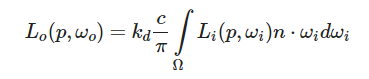
2,IBL 照明:
同样分为两部分,第一部分为direct diffuse lighting。
首先在Diffuse irradiance渲染部分:

本来的解决方案如下:
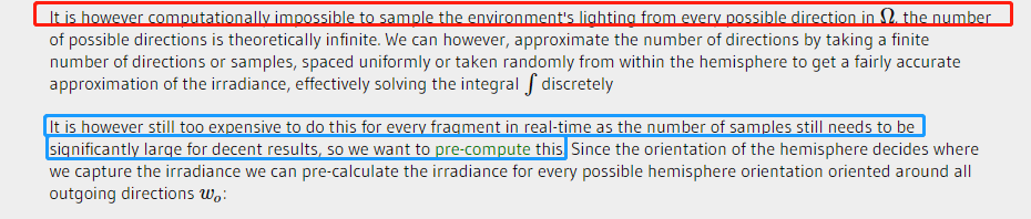
意思就是在半球范围内蒙特卡洛积分,但是问题是在fragment shader 运算这个非常耗时。蓝色的最后pre-compute预计算,预计算就是你拿到的HDR图片的
的辐射度,实际上是蒙特卡洛积分,那么如果我先给你这个方向上的HDR Li辐射度呢?
然后反着看这个方法:
其中Li是最麻烦的,他是任意Wi,dw上的辐射度。为了实时的获取辐射度核心理念就是将N作为获取能量的方向,但是Li是卷积处理过的环境贴图(但是这个环境贴图一定不是模糊贴图那么随便)。
// calculate reflectance at normal incidence; if dia-electric (like plastic) use F0
// of 0.04 and if it's a metal, use the albedo color as F0 (metallic workflow)
vec3 F0 = vec3(0.04);
F0 = mix(F0, albedo, metallic);


vec3 kS = fresnelSchlick(max(dot(N, V), 0.0), F0);
vec3 kD = 1.0 - kS;
kD *= 1.0 - metallic;
vec3 irradiance = texture(irradianceMap, N).rgb;
vec3 diffuse = irradiance * albedo;
vec3 ambient = (kD * diffuse) * ao;
// vec3 ambient = vec3(0.002);

vec3 color = ambient + Lo;

计算半球内的p辐射度的蒙特卡洛法等于对cubemap求卷积。所以教程也是先是HDR->Framebuffer rendering CubeMap->convoluting this cubemap-> 采样在N
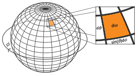
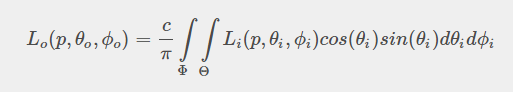
上面的漫反射公式用球坐标是等价意义:
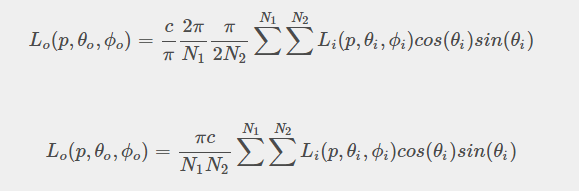
离散后: 注意样本是在phi和theta上分布了N1, N2 个样本 。所以总样本在分母上的话一定N1 * N2
卷积代码:这个是要用framebuffer + colorAttachment ,把结果储存在colorAttachment,在pbr shader 里再samplerCube回来。
#version 330 core
layout (location = 0) in vec3 aPos;

out vec3 WorldPos;

uniform mat4 projection;
uniform mat4 view;

void main()
{
    WorldPos = aPos;
    gl_Position =  projection * view * vec4(WorldPos, 1.0);
}
#version 330 core
out vec4 FragColor;
in vec3 WorldPos;

uniform samplerCube environmentMap;

const float PI = 3.14159265359;

void main()
{
    // The world vector acts as the normal of a tangent surface
    // from the origin, aligned to WorldPos. Given this normal, calculate all
    // incoming radiance of the environment. The result of this radiance
    // is the radiance of light coming from -Normal direction, which is what
    // we use in the PBR shader to sample irradiance.
    vec3 N = normalize(WorldPos);

    vec3 irradiance = vec3(0.0);

    // tangent space calculation from origin point
    vec3 up    = vec3(0.0, 1.0, 0.0);
    vec3 right = cross(up, N);
    up            = cross(N, right);

    float sampleDelta = 0.025;
    float nrSamples = 0.0;
    for(float phi = 0.0; phi < 2.0 * PI; phi += sampleDelta)
    {
        for(float theta = 0.0; theta < 0.5 * PI; theta += sampleDelta)
        {
            // spherical to cartesian (in tangent space)
            vec3 tangentSample = vec3(sin(theta) * cos(phi),  sin(theta) * sin(phi), cos(theta));
            // tangent space to world
            vec3 sampleVec = tangentSample.x * right + tangentSample.y * up + tangentSample.z * N;

            irradiance += texture(environmentMap, sampleVec).rgb * cos(theta) * sin(theta);
            nrSamples++;
        }
    }
    irradiance = PI * irradiance * (1.0 / float(nrSamples));

    FragColor = vec4(irradiance, 1.0);
最后pbr shader代码获取这个就简单了:
vec3 irradiance = texture(irradianceMap, N).rgb;
vec3 diffuse = irradiance * albedo;
在这里如果有2个物体,相互之间有遮挡,这样简单的判断,实际上物体相互之间的遮挡的环境辐射度肯定低,在Raytracing框架却很容易实现,当前作者并没有考虑此问题
Specular IBL:

这次积分的BRDF 依靠 wi wo n向量,不像diffuse ibl只依靠wi,解决方案就是Epic Games' split sum approximation :
积分第一个部分是 pre-filtered environment map (预计算/过滤环境贴图),similar to the diffuse irradiance map
这个和diffuse环境贴图卷积是不一样,要考虑下roughness,因为一定要模拟在microface表面的一个效果:
第一幅图就是个镜面反射比较简单。也就是在我们的方案中,不卷积环境贴图,roughness为0。
后面2个高光采样的话有2中方案把采样分布到 Lobe中,参见我以前的文章:ImportanceSampleGGX && "CosWeightedSampleGGX"
作者相应的卷积公式第一部分代码:
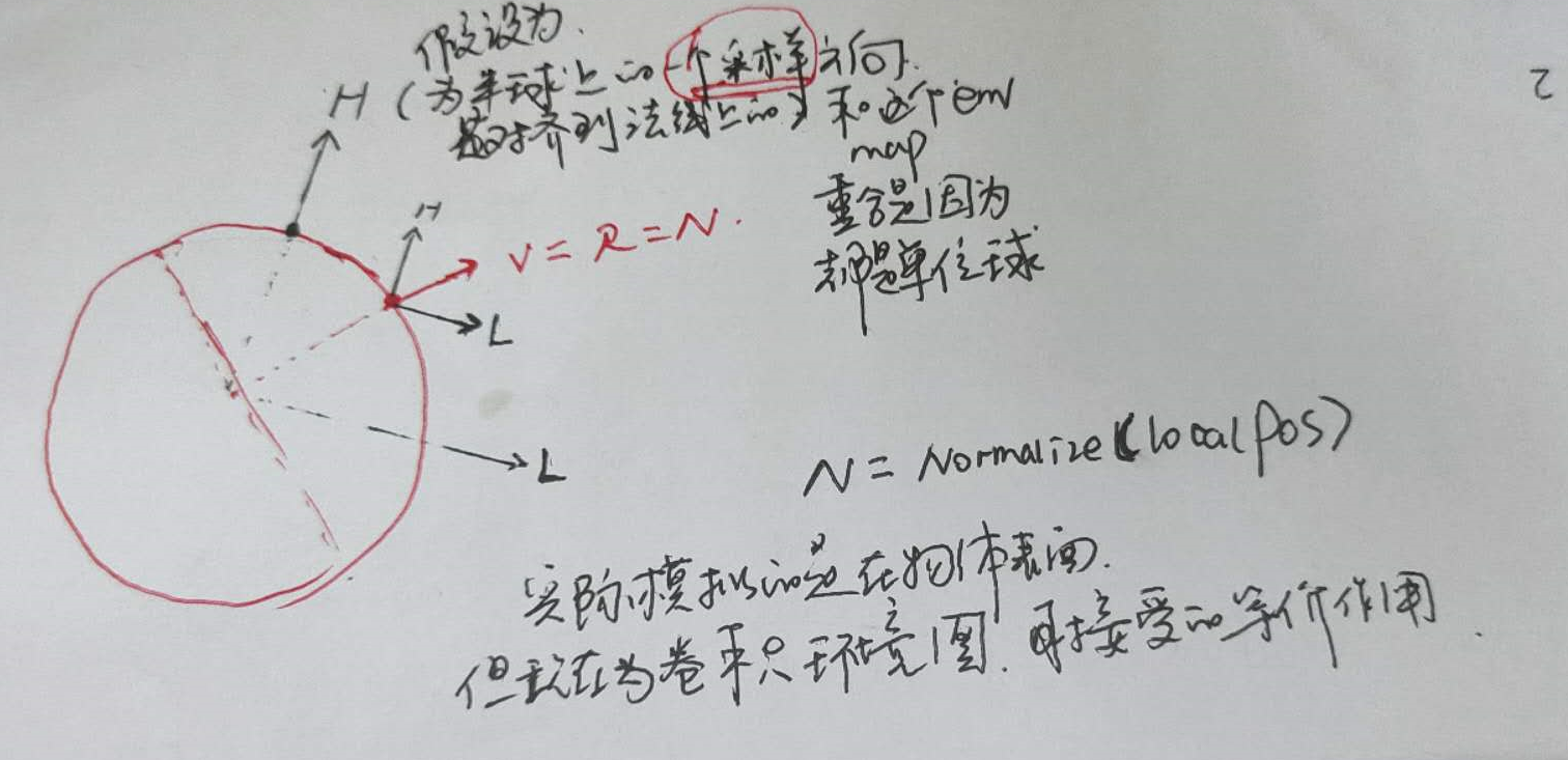
#version 330 core
out vec4 FragColor;
in vec3 localPos;

uniform samplerCube environmentMap;
uniform float roughness;

const float PI = 3.14159265359;

float RadicalInverse_VdC(uint bits);
vec2 Hammersley(uint i, uint N);
vec3 ImportanceSampleGGX(vec2 Xi, vec3 N, float roughness);

void main()
{
    vec3 N = normalize(localPos);
    vec3 R = N;
    vec3 V = R;

    const uint SAMPLE_COUNT = 1024u;
    float totalWeight = 0.0;
    vec3 prefilteredColor = vec3(0.0);
    for(uint i = 0u; i < SAMPLE_COUNT; ++i)
    {
        vec2 Xi = Hammersley(i, SAMPLE_COUNT);
        vec3 H  = ImportanceSampleGGX(Xi, N, roughness);
        vec3 L  = normalize(2.0 * dot(V, H) * H - V);

        float NdotL = max(dot(N, L), 0.0);
        if(NdotL > 0.0)
        {
            prefilteredColor += texture(environmentMap, L).rgb * NdotL;
            totalWeight      += NdotL;
        }
    }
    prefilteredColor = prefilteredColor / totalWeight;

    FragColor = vec4(prefilteredColor, 1.0);
}
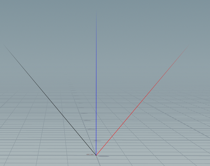
其中:如上图我画的向量解释:
vec3 L = normalize(2.0 * dot(V, H) * H - V);
V向量是红色(在卷积贴图中认为的由点位置到摄像机向量),H向量是蓝色(GGX重要性采样向量),L向量为黑色(反射向量)。可以试着想下 在卷积环境球表面的情况。
为了更加简化这个过程,教程中使用的是Cube Map,我想如果换成HDR Image -> 卷积 - >HDR Sphere。那岂不是更简单:
所以一切的方案首先从houdini实践正确性。而且顺便测试了离线的HDR sphere这种方式,而不是用cube map的这种傻逼方式(在这里不管任何性能):

所以我的思路实现方法:给你一个图片,先把他卷积了,在houdini卷积就是直接用comp系统(opengl对应framebuffer color attachment)
但是houdini comp里首先得把uv坐标转换成一个球坐标。这里公式来自于PBRT
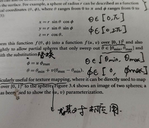
第一幅图是把uv转sphere的坐标:
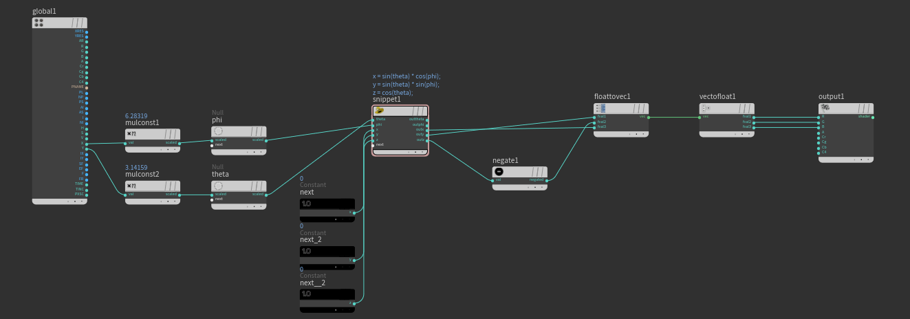
snippt代码:
x = sin(theta) * cos(phi);
y = sin(theta) * sin(phi);
z = cos(theta);
后面的球坐标xyz要调换下,我对了下单位球位置的顶点颜色,这个是正确的。
第二个comp节点是卷积:

snippt代码:
float roughness = rough;

float VanDerCorpus(int n; int base)
{
    float invBase = 1.0f / float(base);
    float denom   = 1.0f;
    float result  = 0.0f;

    for(int i = 0; i < 32; ++i)
    {
        if(n > 0)
        {
            denom   = float(n) % 2.0f;
            result += denom * invBase;
            invBase = invBase / 2.0f;
            n       = int(float(n) / 2.0f);
        }
    }

    return result;
}
// ----------------------------------------------------------------------------

// ----------------------------------------------------------------------------
vector2 HammersleyNoBitOps(int i; int N)
{
    return set(float(i)/float(N), VanDerCorpus(i, 2));
}


vector ImportanceSampleGGX(vector2 Xi;vector N;float roughness)
{
    float a = roughness*roughness;

    float phi = 2.0 * PI * Xi.x;
    float cosTheta = sqrt((1.0 - Xi.y) / (1.0 + (a*a - 1.0) * Xi.y));
    float sinTheta = sqrt(1.0 - cosTheta*cosTheta);

    // from spherical coordinates to cartesian coordinates
    vector H;
    H.x = cos(phi) * sinTheta;
    H.y = sin(phi) * sinTheta;
    H.z = cosTheta;

    // from tangent-space vector to world-space sample vector
    vector up        = abs(N.z) < 0.999 ? set(0.0, 0.0, 1.0) : set(1.0, 0.0, 0.0);
    vector tangent   = normalize(cross(up, N));
    vector bitangent = cross(N, tangent);

    vector sampleVec = tangent * H.x + bitangent * H.y + N * H.z;
    return normalize(sampleVec);
}


vector sampleSphere(vector dir; string img){
    float phi = atan2(dir.x, dir.z);
    float theta = acos(dir.y);
    float u = phi / (2.000 *PI );
    float v = 1 - theta / PI;
    //u = clamp(u,0,1);
    //v = clamp(v,0,1);
    vector imgL = texture(img,u,v);
    return imgL;
}


int SAMPLE_COUNT = count;
vector N = normalize(localPos);
vector R = N;

vector V = R;
float totalWeight = 0.0;
vector prefilteredColor = 0.0;

for(int i = 0; i < SAMPLE_COUNT; ++i)
{
    int testi = i;
    vector2 xy = HammersleyNoBitOps(testi,SAMPLE_COUNT);

    vector H  =  ImportanceSampleGGX(xy, N, roughness*roughness);
    vector L  = normalize(2.0 * dot(V, H) * H - V);

    float NdotL = max(dot(N, L), 0.0);
    if(NdotL > 0.0)
    {
        prefilteredColor += sampleSphere(L,map) * NdotL;
        totalWeight      += NdotL;
    }

}


prefilteredColor = prefilteredColor / totalWeight;

color = prefilteredColor;
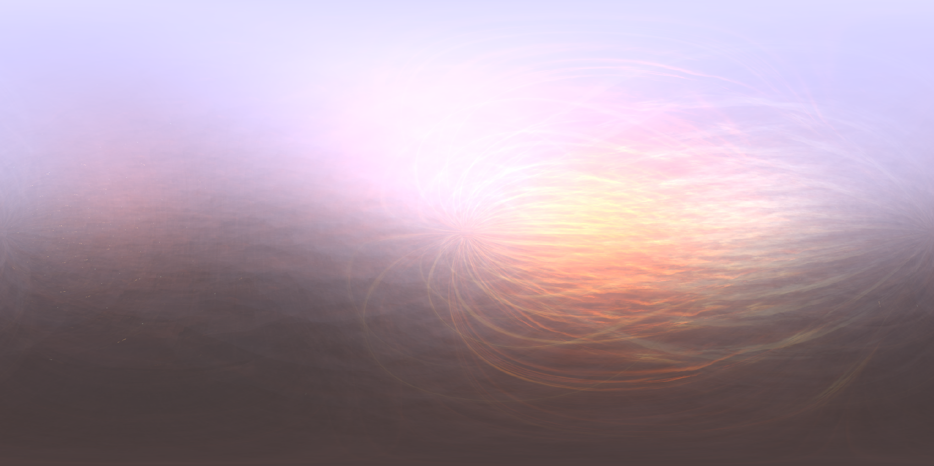
HDR原图:

卷积后结果: samplers:100, roughness:0.7
对应的结果:

roughness:0.1 sampler=100

REF:
https://wiki.jmonkeyengine.org/jme3/advanced/pbr_part3.html#thanks-epic-games
https://learnopengl.com/#!PBR/Theory
http://www.codinglabs.net/article_physically_based_rendering_cook_torrance.aspx
http://www.codinglabs.net/article_physically_based_rendering.aspx

 浙公网安备 33010602011771号