论文解析 -- TPC-H Analyzed: Hidden Messages and Lessons Learned from an Influential Benchmark
该论文主要的目的是,讨论TCPH中的Choke points,
Chokepoints are those technological challenges underlying a benchmark, whose resolution will significantly improve the performance of a product.
Aggregation Performance
由于有lineitem表,通过group_by orderkey,统计订单的信息成为常见的操作
Aggregations occur in all TPC-H queries, hence performance of group-by and aggregation is quite important.
CP1.1: Ordered Aggregation.
HashAgg在HashTable小的情况下,性能最优;
但是当HashTable变大时,性能会分两级退化,首先是无法fit CPU cache,导致lookup更费CPU;当大到RAM无法方向,需要先按hash spill到多个文件,再把每个文件加载到Ram中进行Agg,就无明显性能优势。
如果本身group-by keys是有序的,或者相等的group-by keys是连续的,那么SortAgg会更加合理。
Aggregation implementations typically use a hash-table to store the group-by keys in.
This is an efficient method, because hash-lookup (with a properly sized hash-table) has constant lookup cost.
Hash-aggregation does run into performance deterioration(恶化) when the amount of distinct group-by keys is large.
When the hash-table will no longer fit the various CPU cache levels, cache and TLB misses will make the lookup more costly CPU-wise.
With even more distinct keys, one may get to the situation that the hash-table cannot be kept in RAM anymore.
Here a spilling hash aggregation would be needed, that first hash-partitions the tuple stream to different files based on the hash value, and then aggregates the individual les inside RAM one-at-a-time.
Spilling hash aggregations are not obviously superior to other methods, such as those based on creating a B-tree or, more plausibly(看似合理), those based on sorting (external memory sort).
In case the group-by keys arrive in sorted order, or actually much more generally, if all equal group-by keys appear consecutively(连续的)in the stream, one should employ ordered aggregation instead of hash aggregation.
还有Mix的方法,
These approaches can even be mixed, e.g., using repetitive grouped execution of hash-aggregation, or using hash-based early aggregation in a sort-based spilling approach.
挑战是决定如何选择这些方法,可用硬件,查询数据的特性
关键是要评估中间结果的大小,比如HashTable的大小
Therefore the key challenge is detecting which situation applies, which depends both on the available hardware and the query characteristics.
Related to this, the query optimizer has to infer the correct intermediate result cardinalities, which is relatively simple for most TPC-H query constructs, but challenging for group-by expressions.
CP1.2: Interesting Orders.
如果有序,那么选择SortAgg就是合理的选择
实际情况中,比如对于clustered indexed的字段是天然有序的
除此,某些算子也能做到保序,这里的例子是,当join后面跟着agg的时候,
如果对于Hash Join,其实现是,顺序读probe side的表和build的hash table进行匹配,
所以如果Orders作为probe side,读出的数据是天然按照clustered indexed排序的,即按照o_orderkey有序,
这样紧接着的agg,就可以自然的选择sortAgg。
Apart from clustered indexes providing key order, other operators also preserve or even induce(导致) tuple orderings.
Sort-based operators create new orderings, typically the probe-side of a hash join conserves its order, etc.
For instance TPC-H Q3,4,18 join ORDERS and LINEITEM, followed by aggregation grouped-by on o_orderkey.
If the tuple order of ORDERS is conserved by the join, ordered aggregation is applicable.
This is not to say that it is always best to use the join order with ORDERS on the probe side and LINEITEM on the build side (in hash-join terms),
but if this is chosen then the ordered aggregation benefit should be reaped.
A similar opportunity arises in Q21 with a join between SUPPLIER and LINEITEM, and grouped-by on s_suppkey.
These are an examples of interesting order handling where the query optimization space should take multiple orders into account [3] (i.e. choosing a particular join methods leads to lower aggregation cost, subsequently).
CP1.3: Small Group-By Keys.
groupby的keys的很少的情况下,比如都是性别,flag这种,可以用数组替代HashTable,数组的好处是对cache更友好
Q1 computes eight aggregates: a count, four sums and three averages.
Group-by keys are l_returnflag, l_linestatus, with just four occurring value combinations.
This points to a possibility to optimize a special case of group-by.
Namely, if all group-by expressions can be represented as integers in a small range, one can use an array to keep the aggregate totals by position, rather then keeping them in a hash-table.
This can be extended to multiple group-by keys if their concatenated(串联) integer representation is still "small".
In case of Q1, the group-by attributes are single-characters strings (VARCHAR(1)) which can be stored as an integer e.g. holding the Unicode value.
CP1.4: Dependent Group-By Keys.
GroupBy的key之间存在Functional dependency.
这个在Q10中最明显,可以推导和排除那些依赖的字段,降低cpu和内存的消耗。
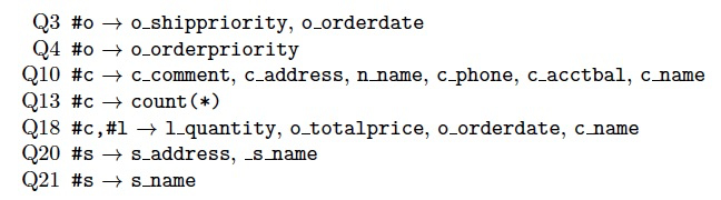
Q10 has an group-by on c_custkey and the columns c_comment, c_address, n_name, c_phone, c_acctbal, c_name.
The amount of data processed is large, since the query involves a one-year ORDERS and LINEITEM join towards CUSTOMER.
Given that c_custkey is the primary key of CUSTOMER, the query optimizer can deduce that its value functionally determines the columns c comment, c address, n name, c phone, c acctbal, c name.
As a result, the aggregation operator should have the ability to exclude certain group-by attributes from key matching: this can greatly reduce the CPU cost and memory footprint of such an operator.
This opportunity arises in many other queries that have an aggregation that includes a tuple identity (denoted #) in addition to other columns that are functionally determined by it:
Join Performance
CP2.1: Large Joins.
HashJoin和Index Join,如何选择,取决于算法的实现和数据库的设计;
总体而言,当join key可以用索引的时候,会选择index join,把有索引的放在内表,对于外表遍历一遍,每个key,查询index获取对应的row。
索引是clustered或unclustered,会涉及到回表的代价,所以如果unclustered索引,用index join意义不大;除非是内存数据库,那么回表的代价可以忽略
Joins are the most costly relational operators, and there has been a lot of research and different algorithmic variants proposed.
Generally speaking, the basic choice is between hash- and index-based join methods.
It is no longer assumed that hash-based methods are always superior to index-based methods;
the choice between the two depends on the system implementation of these methods, as well as on the physical database design:
in general, index-based join methods are used in those situations where the data is stored in an index with a key of which the join key is a prefix.
For the cost model, whether the index is clustered or unclustered makes a large difference in systems relying on I/O;
but (as by now often is the case) if the TPC-H workload hot-set fits into the RAM, the unclustered penalty may be only moderate.
Q9,Q18是large join的例子,在最大的ORDERS和LINEITEM表join上没有过滤的谓词
比如Q9,LINEITEM要和 ORDERS and PARTSUPP join
LINEITEM和 ORDERS,可以按orderKey划分,利用locality的partitioned join;或者如果两表的orderKey都是clustered indexing,可以merge join
但是LINEITEM和PARTSUPP,却没有这样的便利,所以Q9用于测试out-of-core join的性能,比如spilling hash-joins。
同时,这个join需要大量数据shuffle,这个很容易形成性能瓶颈,单纯对于TCPH的测试,可以把PARTSUPP , PART and SUPPLIER副本到每个节点,但这个在实际应用中是不现实的,维护成本太高,除非这些表很少变动。
Q13,可以使用GroupJoin operator,避免两次建立hash table。
Q9 and Q18 are the queries with the largest joins without selection predicates between the largest tables ORDERS and LINEITEM .
The heaviest case is Q9, which essentially joins it also with PARTSUPP , PART and SUPPLIER with only a 1 in 17 selection on PART .
The join graph has the largest table LINEITEM joining with both ORDERS and PARTSUPP .
It may be possible to get locality on the former join, using either clustered indexing or table partitioning;
this will create a merge-join like pattern, or a partitioned join where only matching partitions need to be joined.
However, using these methods, the latter join towards the still significantly large PARTSUPP table will not have locality.
This lack of locality causes large resource consumption, thus Q9 can be seen as the query that tests for out-of-core join methods (e.g. spilling hash-joins).
In TPC-H, by configuring the test machine with sufficient RAM, typically disk spilling can be avoided, avoiding its high performance penalty.
In the case of parallel database systems, lack of join locality will cause unavoidable network communication, which quickly can become a performance bottleneck.
Parallel database systems can only avoid such communication by replicating the PARTSUPP , PART and SUPPLIER tables on all nodes a strategy
which increases memory pressure and disk footprint, but which is not penalized by extra maintenance cost, since the TPC-H refresh queries do not modify these particular tables.
For specific queries, usage of special join types may be beneficial.
For example, Q13 can be accelerated by the GroupJoin operator [4], which combines the outer join with the aggregation and thus avoids building the same hash table twice.
CP2.2: Sparse Foreign Key Joins.
除Q1,6,其他的Q都是join;除Q9和Q18,在join之前对于数据都有严格的谓词筛选,所以导致在 N:1 or 1:N的join中,产生稀疏foreign key的情况;
比如Q2,在对Part进行过滤后,剩下的Part可能就是个位数
这里的优化,就是对于产生稀疏foreign key的side,动态生成bloom filter,然后在Probe过程中,将其下推到另一个side的Scan,降低数据读取和传输的量。
Joins occur in all TPC-H queries except Q1, 6; and they are invariably(总是) over N:1 or 1:N foreign key relationships.
In contrast to Q9 and Q18, the joins in all other queries typically involve selections; very frequently the :1 side of the join is restricted by predicates.
This in turn means that tuples from the N: side, instead of finding exactly one join partner, often find no partner at all.
In TPC-H it is typical that the resulting join hit-ratios are below 1 in 10, and often much lower.
This makes it beneficial for systems to implement a bloom filter test inside the join [5];
since this will eliminate the great majority of the join lookups in a CPU-wise cheap way, at low RAM investments.
For example, in case of VectorWise, bloom filters are created on-the-fly if a hash-join experiences a low hit ratio,
and make the PARTSUPP-PART join in Q2 six times faster, accelerating Q2 two-fold(双重) overall.
Bloom filters created for a join should be tested as early as possible, potentially before the join, even moving it down into the probing scan.
This way, the CPU work is reduced early, and column stores may further benefit from reduced decompression cost in the scan and potentially also less I/O, if full blocks are skipped [6].
Bloom filter pushdown is furthermore essential in MPP systems in case of such low hit-ratio joins.
The communication protocol between the nodes should allow a join to be preceded by a bloom filter exchange;
before sending probe keys over the network in a communicating join, each local node first checks the bloom filter to see if it can match at all.
In such way, bloom filters allow to significantly bring down network bandwidth usage, helping scalability.
CP2.3: Rich Join Order Optimization.
复杂join order,不同的顺序会产生量级的差别;除了inner,对于semi,anti,outer无法随便的reorder,介绍了一些通用的方法;
TPC-H has queries which join up to eight tables with widely varying cardinalities.
The execution times of different join orders differ by orders of magnitude.
Therefore, finding an efficient join order is important, and, in general, requires enumeration of all join orders, e.g., using dynamic programming.
The enumeration is complicated by operators that are not freely reorderable like semi, anti, and outer joins.
Because of this difficulty most join enumeration algorithms do not enumerate all possible plans, and therefore can miss the optimal join order.
One algorithm that can properly handle semi-, anti-, and outer-joins was developed by IBM for DB2 [7].
Moerkotte and Neumann [8] presented a more general algorithm based on hypergraphs, which supports all relational operators and, using hyperedges, supports join predicates between more than two tables.
CP2.4: Late Projection.
对于列存,有些列到后面才用到,开始可以不读,最后用到的时候,再用rowid读出来
这样的好处,显然中间结果会变小,而且查询越往上可能结果集越小,最终读的数据可能会比较小,比如经过groupby,或topn。
但是也是有损耗的,最终的点查,性能肯定是低于顺序读的,如果最终数据集比较大就得不偿失。
在join中也可以使用late project,join match的时候先只读join keys
In column stores, queries where certain columns are only used late in the plan, can typically do better by omitting them from the original table scans,
to fetch them later by row-id with a separate scan operator which is joined to the intermediate query result.
Late projection does have a trade-off involving locality, since late in the plan the tuples may be in a different order,
and scattered I/O in terms of tuples/second is much more expensive than sequential I/O.
Late projection specifically makes sense in queries where the late use of these columns happens at a moment where the amount of tuples involves has been considerably reduced;
for example after an aggregation with only few unique group-by keys, or a top-N operator.
There are multiple queries in TPC-H that have such pattern, the most clear examples being Q5 and Q10.
A lightweight form of late projection can also be applied to foreign key joins, scanning for the probe side first only the join keys, and only in case there is a match,
fetching the remaining columns (as mentioned in the bloom filter discussion).
In case of sparse foreign key joins, this will lead to reduced column decompression CPU work, and potentially also less I/O - if full blocks can be skipped.
Data Access Locality
TCPD到TCPD和TCPH的演变,TCPH不支持物化视图
A popular data storage technique in data warehousing is the materialized view.
Even though the TPC-H workload consists of multiple query runs, where the 22 TPC-H queries are instrumented with different parameters,
it is possible to create very small materialized views that basically contain the parameterized answers to the queries.
Oracle issued in 1998 the One Million Dollar Challenge, for anyone who could demonstrate that Microsoft SQL server 7.0 was not 100 times slower than Oracle when running TPC-D;
exploiting the fact that Oracle had introduced materialized views before SQL server did.
Since materialized views essentially turn the decision support queries of TPC-D into pre-calculated result-lookups, the benchmark no longer tested ad-hoc query processing capabilities.
This led to the split of TPC-D into TPC-R (R for Reporting, now retired, where materialized views were allowed), and TPC-H, where materialized views were outlawed.
As such, even though materialized views are an important feature in data warehousing, TPC-H does not test their functionality.
CP3.1: Columnar Locality.
列存,对于TCPH,有一半的数据大小在comment字段,所以用列存对TCPH的性能提升是显著的
The original TPC-D benchmark did not allow the use of vertical partitioning.
However, in the past decade TPC-H has been allowing systems that uniformly vertically partition all tables ("column stores").
Columnar storage is popular as it accelerates many analytical workloads, without relying on a DBA to e.g. carefully choose materialized views or clustered indexes.
As such, it is considered a more "robust" technique.
The main advantage of columnar storage is that queries only need to access those columns that actually are used in a query.
Since no TPC-H query is of the form SELECT * FROM .., this benefit is present in all queries.
Given that roughly half of the TPC-H data volume is in the columns l_comment and o_comment (in VectorWise),
which are very infrequently accessed, one realizes the benefit is even larger than the average fraction of columns used by a query.
Not only do column-stores eliminate unneeded I/O, they also employ effective columnar compression, and are best combined with an efficient query compiler or execution engine.
In fact, both the TPC-H top-scores for cluster and single-server hardware platforms in the years 2010-2013 have been in the hands of columnar products (EXASOL and VectorWise).
CP3.2: Physical Locality by Key.
字段之间,有时候存在关联性,比如在TCPH中,各种date的生成是强相关的
那么这样从一个字段的筛选谓词,就可以推断出其他字段的选项谓词,即谓词推导
比如对于Q3,虽然只明确写了orderdate的HI,但是从shipdate的LO,也能推导出orderdate的LO,这样就可以更加有效的过滤order
这个前提是,优化器要能够感知到这种关联,这个往往在实践中不是那么容易的
The TPC-H tables ORDERS and LINEITEM contain a few date columns, that are correlated by the data generator:
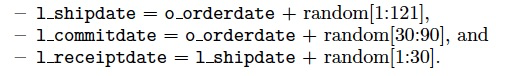
In Q3, there is a selection with lower bound (LO) on l_shipdate and a higher bound (HI) on o_orderdate .
Given the above, one could say that o_orderdate is thereby restricted on the day range [LO-121:HI].
Similar bounds follow for any of the date columns in LINEITEM .
The combination of a lower and higher bound from different tables in Q3 is an extreme case,
but in Q4,5,8,10,12 there are range restrictions on one date column, that carry over to a date restriction to the other side of the ORDERS -LINEITEM join.
Clustered Indexes.
如果在Join的时候,用有关联性性字段,分别用作clustered index,那么读出的数据都是几乎有序的,类似merge join的性能;
It follows that storing the ORDERS relation in a clustered index on o_orderdate and LINEITEM on a clustered index on any of its date columns;
in combination with e.g. unclustered indexes to enforce their primary keys, leads to joins that can have high data locality.
Not only will a range restriction save I/O on both scans feeding into the join, but in a nested-loops index join the cursor will be moving in date order through both tables quasi-sequentially(几乎是顺序);
even if the access is by the orderkey via an unclustered index lookup. Such an unclustered index could easily be RAM resident and thus fast to access.
In Q3,4,5,8,10,12 the date range selections take respectively 2,3,12,12,3,12 out of 72 months.
Typically this 1 in 6 to 1 in 36 selection fraction on the ORDERS table is propagable to the large LINEITEM table, providing very significant benefits.
In Q12 the direction is reverted: the range predicate is on l_receiptdate and can be propagated to ORDERS (similar actually happens in Q7, here through l_shipdate ).
Even though this locality automatically emerges during joins if ORDERS and LINEITEM both are stored in a clustered index with a date key,
the best plan might not be found by the optimizer if it is not aware of the correlation.
Microsoft SQL server specifically offers the DATE_CORRELATION_OPTIMIZATION setting that tells the optimizer to keep correlated statistics.
Table Partitioning.
Partitioning对于TCPH,主要的作用是pruning;由于TPCH没有显式的索引创建,所以了解partitions之间的correlation,比如通过pruning bitmap,可以更好的pruning
Range-partitioning is often used in practice on a time dimension, in which case it provides support for so-called data life-cycle management .
That is, a data warehouse may keep the X last months of data, which means that every month the oldest archived month must be removed from the dataset.
Using range-partitioning, such can be efficiently achieved by range-partitioning the data per month, dropping the oldest partition.
However, the refresh workload of TPC-H does not fit this pattern, since its deletes and inserts are not time-correlated.
The benefit from table partitioning in TPC-H is hence partition pruning ,
which both can happen in handling selection queries (by not scanning those partitions that cannot contain results, given a selection predicate) and in joins between tables that are partitioned on the primary and foreign keys.
Data correlation could be exploited in partitioning as well, even respecting the TPC-H rule that no index creation directive (or any other DDL) would mention multiple tables.
For example, for range-partitioned tables it is relatively easy to automatically maintain for all declared foreign key joins to another partitioned table a pruning bitmap for each partition,
that tells with which partitions on the other side the join result is empty.
Such a pruning bitmap would steer join partition pruning and could be cheaply maintained as a side effect of foreign-key constraint checking.
CP3.3: Detecting Correlation.
仍然讲的是列关联性,通过多维histogram,这个代价比较高
后续提到SMA,MinMax,这个和关联性啥关系?一般用于列存的pruning
While the TPC-H schema rewards creating these clustered indexes, in case of LINEITEM the question then is which of the three date columns to use as key.
One could say that l_shipdate is used more often (in Q6,15,20) than l_receiptdate (just Q12),
but in fact it should not matter which column is used, as range-propagation between correlated attributes of the same table is relatively easy.
One way is through creation of multi-attribute histograms after detection of attribute correlation, such as suggested by the CORDS work in DB2 [9].
Another method is to use small materialized aggregates [10] or even simpler MinMax indexes (VectorWise) or zone-maps (Netezza),
The latter data structures maintain the MIN and MAX value of each column, for a limited number of zones in the table.
As these MIN/MAX are rough bounds only (i.e. the bounds are allowed to be wider than the real data), maintenance that only widens the ranges on need,
can be done immediately by any query without transactional locking.
With MinMax indexes, range-predicates on any column can be translated into qualifying tuple position ranges.
If an attribute value is correlated with tuple position, this reduces the area to scan roughly equally to predicate selectivity.
For instance, even if the LINEITEM is clustered on l receiptdate , this will still find tight tuple position ranges for predicates on l_shipdate (and vice versa).
Expression Calculation
表达式计算,分为纯算术表达式,复杂boolean表达式,字符串匹配
Q1中很多算术表达式,值得被优化
TPC-H tests expression calculation performance, in three areas:
CP4.1: raw expression arithmetic.
CP4.2: complex boolean expressions in joins and selections.
CP4.3: string matching performance.
We elaborate on different technical aspects of these in the following.
Q1 calculates a full price, and then computes various aggregates.
The large amount of tuples to go through in Q1, which selects 99% of LINEITEM, makes it worthwhile to optimize its many arithmetic calculations.
CP4.1a: Arithmetic Operator Performance.
decimals,小数,的表示,用double会损失进度,而且对于SIMD不太友好;用变长的string的话性能太低
According to the TPC-H rules, it is allowed to represent decimals as 64-bits doubles, yet this will lead to limited SIMD opportunities only (4-way in 256-bit AVX).
Moreover, this approach to decimals is likely to be unacceptable for business users of database systems, because of the rounding errors that inevitably appear on "round" decimal numbers.
Another alternative for decimal storage is to use variable-length numerical strings, allowing to store arbitrarily precise numbers;
however in that case arithmetic will be very slow, and this would very clearly show in e.g. Q1.
一种方法是,直接把小数当整数存,这样还需要额外存一下小数点的位置;
TCPH,比较简单,因为对于decimal是有范围限制的,这样不但用64-bits的int可以存下,小数点的位置是固定的;
这个方法问题是,实际情况下,你无法对于小数点后的精度有所假设,这个方法不通用;
而且这个方法仍然需要64-bit,对于SIMD也不友好。
A common and efficient implementation for decimals is to store integers containing the number without dot.
The TPC-H spec states that the decimal type should support the range [-9,999,999,999.99: 9,999,999,999.99] with increments of 0.01.
That way, the stored integer would be the decimal value times 100 and 42-bits of precision are required for TPC-H decimals, hence a 32-bits integer is too small but a 64-bits integer suffices.
Decimal arithmetic can thus rely on integer arithmetic, which is machine-supported and even SIMD can be exploited.
自然想到,每个列其实的取值范围是不同的,不用最大的范围去编码每一列,比如对于discount,8bits就够了,那么一次SIMD可以处理32个tuple,性能就提升了
It is not uncommon for database systems to keep statistics on the minimum and maximum values in each table column.
The columns used in Q1 exhibit the following ranges: l_extendedprice [0.00:100000.00], l_quantity [1.00:50.00], l_discount [0.00:0.10] and l_tax [0.00:0.08].
This means that irrespective of how data is physically stored (columnar systems would typically compress the data),
during query processing these columns could be represented in byte-aligned integers of 32, 16, 8 and 8 bits respectively.
The expression (1-l discount) using an 8-bits representation can thus be handled by SIMD subtraction, processing 32 tuples per 256-bits AVX instruction.
However, the subsequent multiplication with l_extendedprice requires to convert the result of (1-l discount) to 32-bits integers, still allowing 256-bits SIMD multiplication to process 8 tuples per instruction.
This highlights that in order to exploit SIMD well, it pays to keep data represented as long as possible in as small as possible integers (stored column-wise).
Aligning all values on the widest common denominator (the 32-bits extendedprice ) would hurt the performance of four out of the six arithmetic operations in our example Q1; making them a factor 4 slower.
While SIMD instructions are most easily applied in normal projection calculations, it is also possible to use SIMD for updating aggregate totals.
In aggregations with group-by keys, this can be done if there are multiple COUNT or SUM operations on data items of the same width, which then should not be stored column-wise but rather row-wise in adjacent fields [11].
CP4.1b: Overflow Handling.
溢出检查的成本较高,可以通过估算各个字段的取值范围来避免溢出检查
Arithmetic overflow handling is a seldom covered topic in database research literature, yet it is a SQL requirement.
Overflow checking using if-then-else tests for each operation causes CPU overhead, because it is extra computation.
Therefore there is an advantage to ensuring that overflow cannot happen, by combining knowledge of data ranges and the proper choice of data types.
In such cases, explicit overflow check codes that would be more costly than the arithmetic itself can be omitted, and SIMD can be used.
The 32-bits multiplication l_extendedprice*(1-l_discount), i.e. [0.00:100000.00]*[0.00:0.90] results in the more precise value range [0.0000:90000.0000] represented by cardinals up to 900 million;
hence 32-bits integers still cannot overflow in this case. Thus, testing can be omitted for this expression.
CP4.1c: Compressed Execution.
不解压计算,列存中常见,不解压filter,比较或数字计算;这里提到用RLE编码压缩,可以不解压直接做聚合,但是不能groupby。
Compressed execution allows certain predicates to be evaluated without decompressing the data it operates on, saving CPU effort.
The poster-child use case of compressed execution is aggregation on RLE compressed numerical data [12], however this is only possible in aggregation queries without group-by.
This only occurs in TPC-H Q6, but does not apply there either given that the involved l_extendedprice column is unlikely to be RLE compressed.
As such, the only opportunities for compressed execution in TPC-H are in column vs. constant comparisons that appear in selection clauses;
here the largest benefits are achieved by executing a VARCHAR comparison on dictionary-compressed data, such that it becomes an integer comparison.
CP4.1d: Interpreter Overhead
表达式的执行,如果每个tuple都去遍历一遍表达式树,效率太低;
当前通过硬件,JIT编译,向量化执行来提升;思路,提升每次执行效率,硬件或JIT;提升一次执行的tuple数,向量化;AP常用向量化,处理的数据足够多,解释表达式tree的成本就分摊了
The large amount of expression calculation in Q1 penalizes slow interpretative (tuple-at-a-time) query engines.
Various solutions to interpretation have been developed, such as using FPGA hardware (KickFire), GPU hardware (ParStream), vectorized execution (VectorWise) and Just-In-Time (JIT) compilation (HyPer, ParAccel);
typically beating tuple-at-a-time interpreters by orders of magnitude in Q1.
CP4.2a: Common Subexpression Elimination.
公共子表达式消除,避免重复计算
A basic technique helpful in multiple TPC-H queries is common subexpression elimination (CSE).
In Q1, this reduces the six arithmetic operations to be calculated to just four.
CSE should also recognize that two of the average aggregates can be derived afterwards by dividing a SUM by the COUNT, both also computed in Q1.
CP4.2b: Join-Dependent Expression Filter Pushdown.
将join condition中的过滤条件,生成新的过滤算子,进行下推;
Q7的例子,很容易从join condition中推导出,(cn.n name = '[NATION1]' OR cn.n name = '[NATION2]'),提前进行下推
In Q7 and Q19 there are complex join conditions which depend on both sides of the join.
In Q7, which is a join query that unites customer-nations (cn) via orders, lineitems, and suppliers to supplier-nations (sn), and on top of this it selects:
(sn.n name = '[NATION1]' AND cn.n name = '[NATION2]') OR (sn.n name = '[NATION2]' AND cn.n name = '[NATION1]').
Hence TPC-H rewards optimizers that can analyze complex join conditions which cannot be pushed below the join, but still derive filters from such join conditions.
For instance, if the plan would start by joining CUSTOMER to NATION, it could immediate filter the latter scan with the condition:
(cn.n name = '[NATION1]' OR cn.n name = '[NATION2]')
This will reduce data volume with a factor 12.5.
A similar technique can be used on the disjunctive complex expression in Q19.
The general strategy is to take the union of the individual table predicates appearing in the disjunctive condition, and filter on this in the respective scan.
进一步的优化可以将nation的字符串的比较,转化为整形的比较
A further optimization is to rewrite the NATION scans as subqueries in the FROM clause:
(SELECT (CASE n_name = '[NATION1]' THEN 1 ELSE 0 END) AS nation1,
(CASE n_name = '[NATION2]' THEN 1 ELSE 0 END) AS nation2
FROM nation WHERE n_name = '[NATION1]' or n_name = '[NATION2]') cn
And subsequently test the join condition as:
(sn.nation1=1 AND cn.nation2=1) OR (sn.nation2=1 AND cn.nation1=1)
The rationale for the above is that integer tests (executed on the large join result) are faster than string equality.
A rewrite like this may not be needed for (column store) systems that use compressed execution, i.e. the ability to execute certain predicates in certain operators without decompressing data [13].
CP 4.2c: Large IN Clauses.
in clauses,可以转化为一系列的合取范式;但是如果比较多的化,可以转换成hash-table,进行semi-join,这种join称为invisible join
In Q19, Q16 and Q22 (and also Q12) there are IN predicates against a series of at most eight constant values,
though in practice OLAP tools that generate SQL queries often create much bigger IN clauses.
A naive way to implement IN is to map it into a nested disjunctive expression; however this tends to work well with only a handful of values.
In case of many values, performance can typically be won by creating an on-the-fly hash-table, turning the predicate into a semi-join.
This effect where joins turn into selections can also be viewed as a "invisible join" [13].
CP 4.2d: Evaluation Order in Conjunctions and Disjunctions.
对于复杂的and,or过滤谓词,evaluation order会影响性能;
对于X and Y,如果X=false,那么就可以ignore Y,所以应该尽量把选择率小的放左边,但是这样前提是统计是准确的;
甚至OR(x,y),可以被优化成,(NOT(AND(NOT(x),NOT(y)))
In Q19 in particular, but in multiple other queries (e.g. Q6) we see the challenge of finding the optimal evaluation order for complex boolean expressions consisting of conjunctions and disjunctions.
Conjuctions can use eager evaluation, i.e. in case of (X and Y) refrain from computing expression Y if X=false.
As such, an optimizer should rewrite such expressions into Y and X in case X is estimated to be less selective than Y, this problem can be generalized to arbitrarily complex boolean expressions [10].
Estimating the selectivities of the various boolean expressions may be difficult due to incomplete statistics or correlations.
Also, features like range-partitioning (and partition pruning) may interact with the actually experienced selectivities - and in fact selectivities might change during query execution.
For instance, in a LINEITEM table that is stored in a clustered index on l_shipdate, a range-predicate on l_receiptdate typically first experiences a selection percentage of zero,
which at some point starts to rise linearly, until it reaches 100% before again linearly dropping off to zero.
Therefore, there is an opportunity for dynamic, run-time schemes of determining and changing the evaluation order of boolean expressions [14].
In the case of VectorWise a 20% performance improvement was realized in Q19 by making the boolean expression operator sensitive to the observed selectivity in conjunctions, swapping left for right
if the second expression is more selective regularly at run-time - and OR(x,y) being similarly optimized by rewriting it to (NOT(AND(NOT(x),NOT(y))) followed by pushing down the inner NOTs (such that NOT(a > 2) becomes a <= 2).
CP 4.3a: Rewrite LIKE(X%) into Range Query.
Like是很低效的,尤其是对于大的字符串字段;
这里好像也没有啥通用的优化,这里给了Q14,16,20中prefix search的例子,
(LIKE('xxx%')可以变换成性能好些的,(BETWEEN 'xxx' AND 'xxy')
Q2,9,13,14,16,20 contain expensive LIKE predicates; typically, string manipulations are much more costly than numerical calculations;
and in Q13 it also involves l comment, a single column that represents 33% of the entire TPC-H data volume (in VectorWise).
LIKE processing has not achieved much research attention; however relying on regular expression libraries, that interpret the LIKE pattern string (assuming the pattern is a constant) is typically not very efficient.
A better strategy is to have the optimizer analyze the constant pattern.
A special case, is prefix search (LIKE('xxx%') that occurs in Q14,16,20; which can be prefiltered by a less expensive string range comparison (BETWEEN 'xxx' AND 'xxy').
CP4.3b: Raw String Matching Performance.
X86扩展指令集,可以用SIMD来比较编码成16字节的字符串,性能会大幅提升;
但是对于长字符串完整匹配才比较有效果,比如groupby,大量重复的完整匹配
一般字符串匹配,可能在第一二个字符就发现不匹配,会长匹配的概率不大,这种就没有啥优化效果
The x86 instruction set has been extended with SSE4.2 primitives that provide rather a-typical functionality:
they encode 16-byte at-a-time string comparisons in a single SIMD instruction.
Using such primitives can strongly speed up long string comparisons; going through 16 bytes in 4 cycles on e.g. the Nehalem core (this is 20 times faster than a normal strcmp).
However, using these primitives is not always faster, as very short string comparisons that break off at the first or second byte can be better done iteratively.
Note that if string comparisons are done during group-by, as part of a hash-table lookup, they typically find an equal string and therefore have to go through it fully, such that the SSE4.2 implementation is best.
In contrast, string comparisons done as part of a selection predicate might more often fall in the case where the strings are not equal, favoring the iterative approach.
CP4.3c: Regular Expression Compilation.
Complex LIKE expression should best not be handled in an interpretative way, assuming that the LIKE search pattern is a constant string.
The database query compiler could compile a Finite State Automaton (FSA) for recognizing the pattern.
Another approach is to decompose the LIKE expression into a series of simpler functions, e.g. one that searches forward in a string and returns the new matching offset.
This should be used in an iterative way, taking into account backtracking after a failed search.
CP-CorrelatedSubqueries.
CP5.1: Flattening Subqueries.
关联子查询,TPCH中的都可以flatten为join,比如equi-join, outer-join or anti-join
子查询,也可以通过向量化或block-wise来优化,批量可以摊薄所有的成本
Many TPC-H queries have correlated subqueries.
All of these query plans can be flattened, such that the correlated subquery is handled using an equi-join, outer-join or anti-join [15].
In Q21, for instance, there is an EXISTS clause (for orders with more than one supplier) and a NOT EXISTS clauses (looking for an item that was received too late).
To execute Q21 well, systems need to flatten both subqueries, the first into an equi-join plan, the second into an anti-join plan.
Therefore, the execution layer of the database system will benefit from implementing these extended join variants.
The ill effects of repetitive tuple-at-a-time subquery execution can also be mitigated in execution systems use vectorized, or block-wise query execution, allowing to run sub-queries with thousands of input parameters instead of one.
The ability to look up many keys in an index in one API call, creates the opportunity to benefit from physical locality, if lookup keys exhibit some clustering.
CP5.2: Moving Predicates into a Subquery.
关联子查询,是被用于条件谓词的scala子查询(aggregate产生标量),并且outer query的条件大于等于子查询,可以将外查询的谓词也propagate到子查询中
Q2 shows a frequent pattern: a correlated subquery which computes an aggregate that is subsequently used in a selection predicate of a similarly looking outer query ("select the minimum cost part supplier for a certain part").
Here the outer query has additional restrictions (on part type and size) that are not present in the correlated subquery, but should be propagated to it.
Similar opportunities are found in Q17, and Q20.
CP5.3: Overlap between Outer- and Subquery.
当outer包含inner的时候,除了上面的方式,
decorrelation,去关联重写,比如对于Q17, 子查询变成 groupby partkey,0.2 * avg(l_quantity),的派生表,做一次join即可
这种重写不一定是性能好的,如果过滤完part比较少,那么直接执行子查询可能更加高效
In Q2,11,15,17 and Q20 the correlated subquery and the outer query have the same joins and selections.
In this case, a non-tree, rather DAG-shaped query plan [16] would allow to execute the common parts just once,
providing the intermediate result stream to both the outer query and correlated subquery, which higher up in the query plan are joined together (using normal query decorrelation rewrites).
As such, TPC-H rewards systems where the optimizer can detect this and whose the execution engine sports an operator that can buffer intermediate results and provide them to multiple parent operators.
In Q17, decorrelation, selective join push-down, and re-use together result in a speedup of a factor 500 in HyPer.
Parallelism and Concurrency
CP6.1: Query Plan Parallelization.
可以分为单表的并行,基于多线程利用多核的方式,这个要设计新的算子,比如join,比较麻烦;
mpp,基于数据划分的并行,这个是现在基本实用的并行方式,但如果mpp无法做到locality,数据shuffle的代价也非常的高
Query plan parallelization in the multi-core area is currently an open issue.
At the time of this writing, there is active academic debate on how to parallelize the join operator on many-core architectures, with multiple sophisticated algorithms being devised and tested [17].
We can assume that the current generation of industrial systems runs less-sophisticated algorithms, and presumably in the current state may not scale linearly on many-core architectures.
As such, many-core query parallelization, both in terms of query optimization and query execution is an unresolved choke point.
Further, MPP database systems from the very start focused on scaling out; typically relying on table partitioning over multiple nodes in a cluster.
Table partitioning is specifically useful here in order to achieve data locality; such that queries executing in the cluster find much of the data being operated on on the local node already, without need for communication.
Even in the presence of high-throughput (e.g. Infiniband) network hardware, communication bandwidth can easily become a bottleneck.
For CP6, we acknowledge that the query impact color-classification in Table 1 is debatable.
This classification assumes copartitioning of ORDERS and LINEITEM to classify queries using these as medium hard or hard (if other tables are involved as well).
Single-table queries parallelize trivially and are white.
The idea is that with table partitioning, good parallel speedup is achievable, whereas without it this is harder.
Typically, single-server multi-core parallelism does not rely on table partitioning, though it could.
CP6.2: Workload Management.
资源的管理和隔离,云计算,多租户的情况下是个大问题,跑TCPH应该还好
Another important aspect in handling the Throughput test is workload management, which concerns providing multiple concurrent queries
as they arrive, and while they run, with computational resources (RAM, cores, I/O bandwidth).
The problem here is that the database system has no advance knowledge of the workload to come, hence it must adapt on-the-fly.
Decisions that might seem optimal at the time of arrival of a query, might lead to avoidable thrashing if suddenly additional resource-intensive queries arrive.
In the case of the Power test, workload management is trivial: it is relatively easy to devise an algorithm that while observing that maximally one query is active, assigns all resources to it.
For the Throughput run, as more queries arrive, progressively less resources have to be given to the queries, until the point where there are that many queries in the system and each query gets only a single core.
Since paralellism never achieves perfect scalability, in such cases of high load overall, the highest throughput tends to be achieved by running sequential plans in parallel.
Workload management is even more complicated in MPP systems, since a decision needs to be made on (i) which nodes to involve in each query and (ii) how many resources per node to use.
CP6.3: Result Re-use.
A final observation on the Throughput test is that with a high number of streams, i.e. beyond 20, a significant amount of identical queries emerge in the resulting workload.
The reason is that certain parameters, as generated by the TPC-H workload generator, have only a limited amount of parameters bindings (e.g. there are at most 5 different values for region name r name).
This weakness opens up the possibility of using a query result cache, to eliminate the repetitive part of the workload.
A further opportunity that detects even more overlap is the work on recycling [18], which does not only cache final query results, but also intermediate query results of "high worth".
Here, worth is a combination of partial-query result size, partial-query evaluation cost, and observed (or estimated) frequency of the partial-query in the workload.
It is understood in the rules of TPC-H, though, that any form of result caching should not depend on explicit DBMS configuration parameters, but reflect the default behavior of the system, in order to be admissible.
This rule precludes designing query re-use strategies that particularly target TPC-H, rather, such strategies should be beneficial for most of the intended workloads for which the database system was designed.

 浙公网安备 33010602011771号