Reinforcement Learning from Human Feedback(RLHF): TRPO, PPO, DPO

0 Introduction

Terminology

$S$(state), $A$(action), $R$(reward)
$\tau$(trajectory) = ($s_1$,$a_1$,$r_1$,$s_2$,$a_2$,$r_2$,..., $s_H$)
$\pi$(policy)
$r(x,y)$(reward function), $\pi_r$(corresponding optimal policy for $r(x,y)$)
$r^*(x,y)$(ground-truth reward function), $\pi^*$(corresponding optimal policy for $r^*(x,y)$)
$r_\phi(x,y)$(trained reward model), $\pi_\theta$(active model to be trained), $\pi_\text{ref}$(reference model)

On-policy vs. Off-policy

1 Trust Region Policy Optimization(TRPO)

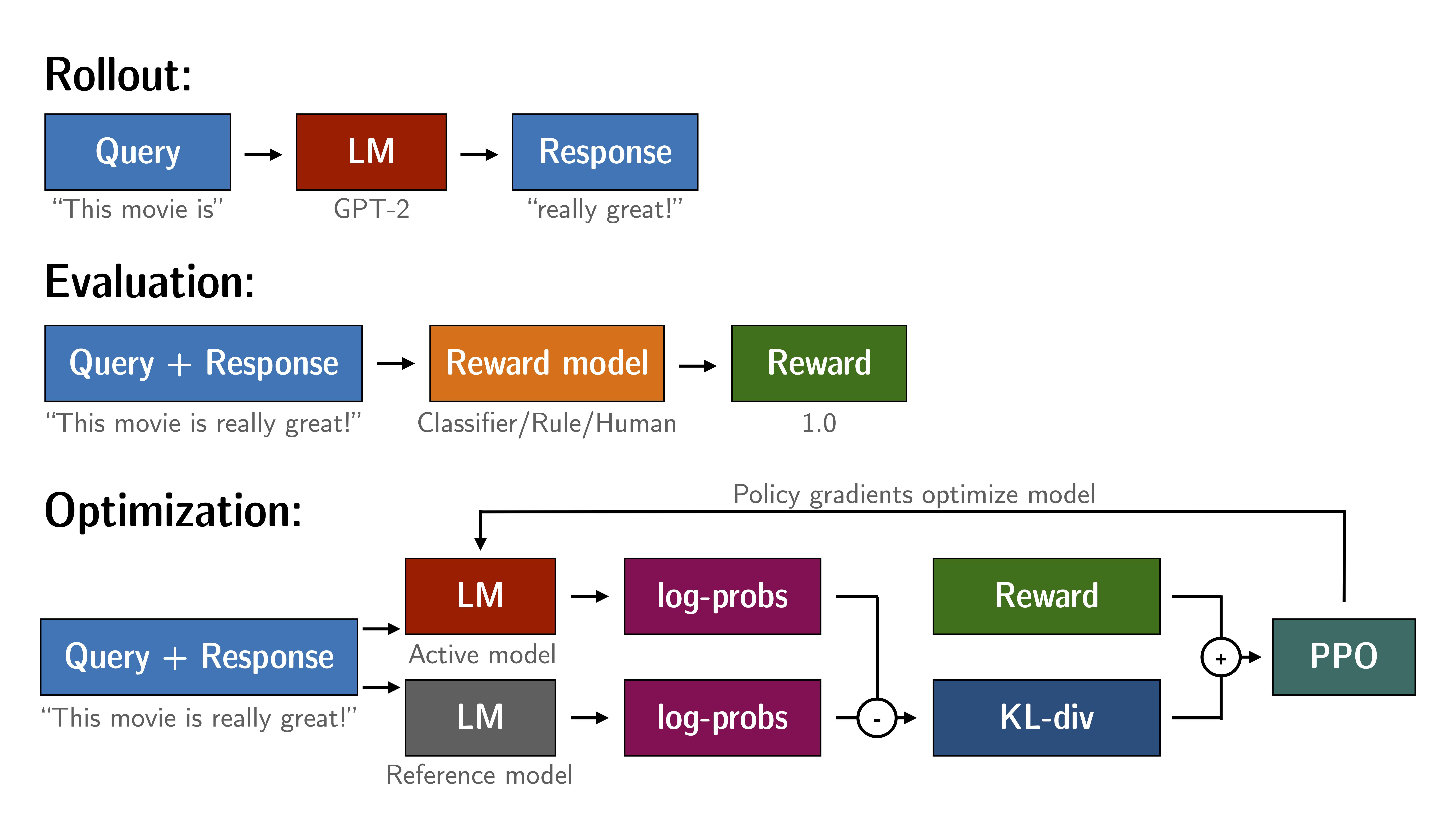
2 Proximal Policy Optimization(PPO)

2.1 Pipeline

<Step 0> Pre-training Language Model Phase, with Self-supervised Learning
The goal is to get the base LLM, which is pre-trained model using tons of unlabeled data.

<Step 1> Supervised Fine-Tuning Language Model Phase
The goal is to make the pre-train model return as the conversation or chat, using the high quality instruction data to train. Save as SFT Language Model.

<Step 2> Reward Modeling Phase
Reward function is to mimic human preference.
Bradley–Terry model

This type of formulation is commonly used in tasks involving pairwise comparisons or ranking.

$p^*(y_1 > y_2 \mid x) = \dfrac{\exp(r^*(x, y_1))}{\exp(r^*(x, y_1)) + \exp(r^*(x, y_2))}$

Loss function(optimization objective to minimize)

$\mathcal{L}_R(r_\phi, D) = -\mathbb{E}_{(x, y_w, y_l) \sim D} \left[ \log \sigma \left( r_\phi(x, y_w) - r_\phi(x, y_l) \right) \right]$

where:

$r_\phi$ is initialized from $\pi^\text{SFT}$ ( = SFT Language Model + nn.Linear(in_features=config.hidden_size,out_features=1,bias=True))

<Step 3> Reinforment Learning Fine-Tuning Phase

Maximizes the reward and prevents the overfitting with KL Divergence Penalty(not too far from the preference language model, not lose the natural language ability)

\begin{align*} \max_{\pi_{\theta}} \mathbb{E}_{x \sim D, y \sim \pi_\theta(y|x)} \left[ r_\phi(x, y)\right] - \beta D_{KL}[\pi_\theta(y|x) \parallel \pi_{\text{ref}}(y|x)] \end{align*}

where:

$\pi_\theta, \pi_\text{ref}$ are initialized from $\pi^\text{SFT}$ ( = SFT Language Model + nn.Linear(in_features=config.hidden_size,out_features=1,bias=True))
$r_{\phi}$ is the trained reward model in the <2> phase

2.2 Mathematical Explanation

2.3 Code

There are three models to use in the implementation:

$r_\phi(x,y)$(trained reward model)
$\pi_\theta$(active model to be trained)
$\pi_\text{ref}$(reference model)

transformers.AutoModelForSequenceClassification

from transformers import AutoModelForSequenceClassification, BitsAndBytesConfig

# Q-LoRA
quantization_config = BitsAndBytesConfig(
    load_in_8bit=False,
    load_in_4bit=True
)

model = AutoModelForSequenceClassification.from_pretrained(
    "facebook/opt-350m",
    quantization_config=quantization_config,
    device_map={"": 0},
    trust_remote_code=True,
    num_labels=1, # out_features = 1
)
model.config.use_cache = False

trl.RewardTrainer

from transformers import TrainingArguments
from peft import LoraConfig
from trl import RewardTrainer

training_args = TrainingArguments(
    output_dir="./train_logs",  
    max_steps=1000,  
    per_device_train_batch_size=4,  
    gradient_accumulation_steps=1,  
    learning_rate=1.41e-5,  
    optim="adamw_torch",  
    save_steps=50,  
    logging_steps=50,  
    report_to="tensorboard",  
    remove_unused_columns=False,  
)

trainer = RewardTrainer(
    model=model,
    tokenizer=tokenizer,
    args=training_args,
    train_dataset=train_dataset,
    peft_config=peft_config,
    max_length=512,
)

trainer.train()

from transformers import AutoModelForCausalLM, AutoTokenizer
from trl import AutoModelForSequenceClassification, PPOConfig, PPOTrainer

# Step 1: Model Instantiation
model = AutoModelForSequenceClassification.from_pretrained("gpt2")
model_ref = AutoModelForSequenceClassification.from_pretrained("gpt2")
tokenizer = AutoTokenizer.from_pretrained("gpt2")
tokenizer.pad_token = tokenizer.eos_token

# Step 2: PPO Trainer
ppo_config = {
    "batch_size": 1
}
config = PPOConfig(**ppo_config)

trainer = PPOTrainer(
    config=config,
    model=model,
    ref_model=model_ref,
    tokenizer=tokenizer
)

3 Direct Preference Optimization(DPO)

3.1 Pipeline

<Step 0> Pre-training Language Model Phase, with Self-supervised Learning
The goal is to get the base LLM, which is pre-trained model using tons of unlabeled data.

<Step 2> DPO Phase

Sample completions $y_1$, $y_2$ ∼ $\pi_\text{ref}(· | x)$ for every prompt x, label with human preferences to construct the offline dataset of preferences $D = \{x^{(i)}, y_w^{(i)} , y_l^{(i)}\}_{i=1}^N$
Optimize the language model $\pi_\theta$ to minimize $\mathcal{L}_{DPO}$ for the given $\pi_\text{ref}$ and $D$ and desired $\beta$. In practice, one would like to reuse preference datasets publicly available, rather than generating samples and gathering human preferences. Since the preference datasets are sampled using $\pi^\text{SFT}$, we initialize $\pi_\text{ref} = \pi^\text{SFT}$ whenever available.
However, when $\pi^\text{SFT}$ is not available, we initialize $\pi_\text{ref}$ by maximizing likelihood of preferred completions ($x$, $y_w$), i.e. $\pi_\text{ref} = arg \max_\pi \mathbb{E}_{x,y_w \sim D} [\log \pi(y_w | x)]$. This procedure helps mitigate the distribution shift between the true reference distribution which is unavailable, and $\pi_\text{ref}$ used by DPO

3.2 Mathematical Explanation

In the RLHF framework, we would like to find the best language model policy that provides the highest reward while still exhibiting similar behavior as expected from the SFT model. This scenario can be mathematically written as the following optimization problem:

\begin{align*} \max_{\pi_{\theta}} \mathbb{E}_{x \sim D, y \sim \pi_\theta(y|x)} \left[ r(x, y)\right] - \beta D_{KL}[\pi_\theta(y|x) \parallel \pi_{\text{ref}}(y|x)] \end{align*}

where

$\pi_\theta, \pi_\text{ref}$ are initialized from $\pi^\text{SFT}$(= SFT Language Model + nn.Linear(in_features=config.hidden_size,out_features=1,bias=True))

Derivation

\begin{align*} & \max_{\pi_{\theta}} \mathbb{E}_{x \sim D, y \sim \pi_\theta(y|x)} \left[ r(x, y)\right] - \beta D_{KL}[\pi_\theta(y|x) \parallel \pi_{\text{ref}}(y|x)] \\ = & \max_{\pi_{\theta}} \mathbb{E}_{x \sim D} \mathbb{E}_{y \sim \pi_{\theta}(y|x)} \left[ r(x, y) - \beta \log \dfrac{\pi_{\theta}(y|x)}{\pi_{\text{ref}}(y|x)} \right] \\ = & \min_{\pi_{\theta}} \mathbb{E}_{x \sim D} \mathbb{E}_{y \sim \pi_{\theta}(y|x)} \left[\log \dfrac{\pi_{\theta}(y|x)}{\pi_{\text{ref}}(y|x)} -\dfrac{1}{\beta}r(x, y) \right] \\ = & \min_{\pi_{\theta}} \mathbb{E}_{x \sim D} \mathbb{E}_{y \sim \pi_{\theta}(y|x)} \left[\log \dfrac{\pi_{\theta}(y|x)}{\pi_{\text{ref}}(y|x)} - \log \exp \left(\dfrac{1}{\beta}r(x, y)\right) \right] \\ = & \min_{\pi_{\theta}} \mathbb{E}_{x \sim D} \mathbb{E}_{y \sim \pi_{\theta}(y|x)} \left[\log \dfrac{\pi_{\theta}(y|x)}{\pi_{\text{ref}}(y|x)} - \log \exp \left(\dfrac{1}{\beta}r(x, y)\right) + \log Z(x) - \log Z(x) \right] \\ = & \min_{\pi_{\theta}} \mathbb{E}_{x \sim D} \mathbb{E}_{y \sim \pi_{\theta}(y|x)} \left[\log \dfrac{\pi_{\theta}(y|x)}{\frac{1}{Z(x)}\pi_{\text{ref}}(y|x)\exp \left(\frac{1}{\beta}r(x, y)\right)} - \log Z(x) \right] \\ = & \min_{\pi_{\theta}} \mathbb{E}_{x \sim D} \mathbb{E}_{y \sim \pi_{\theta}(y|x)} \left[\log \dfrac{\pi_{\theta}(y|x)}{\pi^*(y|x)} - \log Z(x) \right]\\ = & \min_{\pi_{\theta}} \mathbb{E}_{x \sim D} \left[\mathbb{E}_{y \sim \pi_{\theta}(y|x)} \left[\log \dfrac{\pi_{\theta}(y|x)}{\pi^*(y|x)}\right] - \log Z(x) \right] \\ = & \min_{\pi_{\theta}} \mathbb{E}_{x \sim D} \left[ \mathbb{D}_{KL}(\pi_\theta(y|x) \parallel \pi^*(y|x)) - \log Z(x) \right] \end{align*}

where $\mathbb{D}_{KL} \ge 0$, the equal sign holds when $\pi_\theta(y|x) = \pi^*(y|x)$

Now we can define:

\begin{align*} \pi^*(y|x) = \dfrac{1}{Z(x)}\pi_{\text{ref}}(y|x)\exp \left(\dfrac{1}{\beta}r(x, y)\right) \end{align*}

where

$\begin{align*}Z(x) = \sum_y \pi_{\text{ref}}(y|x)\exp \left(\dfrac{1}{\beta}r(x, y)\right)\end{align*}$ is the partition function.
$\pi_{\text{ref}}(y|x)\exp \left(\dfrac{1}{\beta}r(x, y)\right)$ is a valid distribution (probabilities are positive and $\sum_y \pi_{\text{ref}}(y|x)\exp \left(\dfrac{1}{\beta}r(x, y)\right) = 1$)

Hence, we can obtain the ground-truth reward function $r*(x,y)$ explicit expression:

\begin{align*} r^*(x,y) & = \beta \log \left( \dfrac{Z(x)\pi^{*}(y|x)}{\pi_\text{ref}(y|x)} \right)\\ & = \beta \log \dfrac{\pi^*(y|x)}{\pi_\text{ref}(y|x)} + \beta \log Z(x) \end{align*}

Bradley–Terry model

$\begin{align*} p(y_w \succ y_l | x) & = \dfrac{\exp(r^*(x,y_w))}{\exp(r^*(x,y_w)) + \exp(r^*(x,y_l))}\\ & = \dfrac{1}{1 + \exp(r^*(x,y_l) - r^*(x,y_w))}\\ & = \sigma[r^*(x,y_w) - r^*(x,y_l)]\\ & = \sigma \left( \left[ \beta \log \dfrac{\pi^*(y_w | x)}{\pi_{\text{ref}}(y_w | x)} + \beta \log Z(x) \right] - \left[ \beta \log \dfrac{\pi^*(y_l | x)}{\pi_{\text{ref}}(y_l | x)} + \beta \log Z(x) \right] \right)\\ & = \sigma \left( \beta \log \frac{\pi^*(y_w | x)}{\pi_{\text{ref}}(y_w | x)} - \beta \log \frac{\pi^*(y_l | x)}{\pi_{\text{ref}}(y_l | x)} \right) \end{align*}$

Bradley-Terry model can be regraded as the Plackett-Luce model in the paticular condition($K = 2$) over rankings, just pair-wise comparisons.

$\begin{align*} p^*(\tau | y_1, \dots, y_K, x) = \prod_{k=1}^K \dfrac{\exp(r^*(x, y_{\tau(k)}))}{\sum_{j=k}^K \exp(r^*(x, y_{\tau(j)}))} \end{align*}$

Loss function(optimization objective to minimize)

$\begin{align*} \mathcal{L}_{DPO}(\pi_\theta; \pi_{\text{ref}}) & = -\mathbb{E}_{(x,y_w,y_l) \sim D} \left[ \log \sigma \left( \beta \log \frac{\pi_\theta(y_w | x)}{\pi_{\text{ref}}(y_w | x)} - \beta \log \frac{\pi_\theta(y_l | x)}{\pi_{\text{ref}}(y_l | x)} \right) \right] \end{align*}$

DPO update

$ \nabla_\theta \mathcal{L}_{DPO}(\pi_\theta; \pi_{\text{ref}}) = -\beta \mathbb{E}_{(x, y_w, y_l) \sim D} \left[ \sigma \left( \hat{r}_\theta(x, y_l) - \hat{r}_\theta(x, y_w) \right) \left( \nabla_\theta \log \pi(y_w | x) - \nabla_\theta \log \pi(y_l | x) \right) \right] $

where:

$\hat{r}_\theta(x, y) = \beta \log \dfrac{\pi_\theta(y|x)}{\pi_\text{ref}(y|x)}$ is the reward implicitly defined by the language model $\pi_\theta$ and reference model $\pi_\text{ref}$.
$\hat{r}_\theta(x, y_l) - \hat{r}_\theta(x, y_w)$: higher weight when reward estimate is wrong
$\nabla_\theta \log \pi(y_w | x)$: increase likelihood of $y_w$
$\nabla_\theta \log \pi(y_l | x)$: decrease likelihood of $y_l$

Intuitively, the gradient of the loss function $\mathcal{L}_{DPO}$ increases the likelihood of the preferred completions $y_w$ and decreases the likelihood of dispreferred completions $y_l$. Importantly, the examples are weighed by how much higher the implicit reward model $\hat{r}_\theta$ rates the dispreferred completions, scaled by $\beta$, i.e, how incorrectly the implicit reward model orders the completions, accounting for the strength of the KL constraint.

3.3 Code

There are two models to use in the implementation:

$\pi_\theta$(active model to be trained)
$\pi_\text{ref}$(reference model)

import torch.nn.functional as F

def dpo_loss(pi_logps, ref_logps, yw_idxs, yl_idxs, beta):
    """
    pi_logps: policy logprobs, shape (B,)
    ref_logps: reference model logprobs, shape (B,)
    yw_idxs: preferred completion indices in [0, B-1], shape (T,)
    yl_idxs: dispreferred completion indices in [0, B-1], shape (T,)
    beta: temperature controlling strength of KL penalty

    Each pair of (yw_idxs[i], yl_idxs[i]) represents the indices of a single preference pair.
    """
    pi_yw_logps, pi_yl_logps = pi_logps[yw_idxs], pi_logps[yl_idxs]
    ref_yw_logps, ref_yl_logps = ref_logps[yw_idxs], ref_logps[yl_idxs]

    pi_logratios = pi_yw_logps - pi_yl_logps
    ref_logratios = ref_yw_logps - ref_yl_logps
    
    losses = -F.logsigmoid(beta * (pi_logratios - ref_logratios))
    rewards = beta * (pi_logps - ref_logps).detach()

    return losses, rewards

Reference

Paper: Trust Region Policy Optimization
Paper: Proximal Policy Optimization Algorithms
Paper: Direct Preference Optimization: Your Language Model is Secretly a Reward Model
Paper: From r to Q$^∗$: Your Language Model is Secretly a Q-Function

Doc: DPO Trainer - trl | Hugging Face
Doc: PPO Trainer - trl | Hugging Face
Notebook: huggingface/trl/examples/notebooks/gpt2-sentiment.ipynb | GitHub
Video: DRL Lecture 1: Policy Gradient (Review) - Hungyi Lee | Youtube
Video: [pytorch 强化学习] 13 基于 pytorch 神经网络实现 policy gradient（REINFORCE）求解 CartPole - 五道口纳什 | Bilibili
Video: [蒙特卡洛方法] 04 重要性采样补充，数学性质及 On-policy vs. Off-policy - 五道口纳什 | Bilibili
Video: [DRL] 从策略梯度到 TRPO（Lagrange Duality，拉格朗日对偶性） - 五道口纳什 | Bilibili
Video: [personal chatgpt] trl 基础介绍：reward model，ppotrainer - 五道口纳什 | Bilibili
Video: [personal chatgpt] trl reward model 与 RewardTrainer（奖励模型，分类模型） - 五道口纳什 | Bilibili
Video: 构建大语言模型, PPO训练方法, 原理和实现- 蓝斯诺特 | Bilibili
Video: 构建大语言模型, DPO训练方法, 原理和实现- 蓝斯诺特 | Bilibili
Forum: What is the way to understand Proximal Policy Optimization Algorithm in RL? | Stackoverflow
Blog: Forget RLHF because DPO is what you actually need | Medium
Blog: Direct Preference Optimization（DPO）学习笔记 | Zhihu
Blog: DPO 是如何简化 RLHF 的 | Zhihu
Lecture: 10-708: Probabilistic Graphical Models, Spring 2020 | CMU

posted @ 2024-04-16 13:47 ForHHeart 阅读(11) 评论(0) 编辑收藏举报

会员力量，点亮园子希望

刷新页面返回顶部

ForHHeart

Reinforcement Learning from Human Feedback(RLHF): TRPO, PPO, DPO

0 Introduction

Terminology

On-policy vs. Off-policy

1 Trust Region Policy Optimization(TRPO)

2 Proximal Policy Optimization(PPO)

2.1 Pipeline

2.2 Mathematical Explanation

2.3 Code

3 Direct Preference Optimization(DPO)

3.1 Pipeline

3.2 Mathematical Explanation

3.3 Code

Reference

公告