PyTorch Basic Notes
1 Tensors
1.1 Create
1.自定义张量
最左边有几个括号,就是几维向量。
# 一维向量
X1 = torch.tensor([0.0, 1.0, 2.0])
# 二维向量
X2 = torch.tensor([[0., 1., 2.],
                   [3., 4., 5.],
                   [6., 7., 8.]])
# 三维向量
X3 = torch.tensor([[[0., 1., 2.],
                    [3., 4., 5.],
                    [6., 7., 8.]],

                   [[0., 1., 2.],
                    [3., 4., 5.],
                    [6., 7., 8.]],

                   [[0., 1., 2.],
                    [3., 4., 5.],
                    [6., 7., 8.]]])
2.生成全0张量和全1张量
# size为一维张量
X0 = torch.zeros(size)
X1 = torch.ones(size)
3.生成随机数张量
有几个数字,就是几维向量。提高维度只需要在前面加数字。
height为行数,width为列数,channel为通道数,batch为批量。
X1 = torch.rand([4])        # torch.rand(width)
X2 = torch.rand([2,4])      # torch.rand(height, width)
X3 = torch.rand([3,2,4])    # torch.rand(channel, height, width)
X4 = torch.rand([2,3,2,4])  # torch.rand(batch, channel, height, width)
X5 = torch.rand([5,2,3,2,4])# torch.rand(batch, batch, channel, height, width)
4.torch.rand()、torch.randn()、torch.randint()
torch.rand(size) # 返回一个张量,包含了从区间(0,1)的均匀分布中抽取的一组随机数,形状由size决定。
torch.randn(size) # 返回一个张量,包含了从标准正态分布(均值为0,方差为1)中抽取的一组随机数,形状由size决定。
torch.randint(low, high, size) # 返回一个张量,包含了从(low,high)中抽取的一组随机整数,形状由size决定。
torch.arrange(0,10) # tensor([0, 1, 2, 3, 4, 5, 6, 7, 8, 9])
1.2 Multiply
| Traditional Matrix Multiplication(Dot Product) | ||
|---|---|---|
| 1D Tensors (Two vectors) | [n]@[n] = scalar | A@B or torch.dot(A, B) |
| 2D Tensors (Two Matrix) | [m,n]@[n,p] = [m,p] | A@B or torch.mm(A, B) |
| 3D Tensors (Two Batched Matrix) | [b,m,n]@[b,n,p] = [b,m,p] | A@B or torch.bmm(A, B) |
| Higher-dimentional Tensors or Different Dimentional Tensors | [b,m,n]@[n,p] = [b,m,p] | A@B or torch.matmul(A, B) |
| Element-wise Multiplication (Hadamard products) | ||
|---|---|---|
| Tensors (must be the same shape) | [n]@[n] = [n] [m,n]@[m,n] = [m,n] [b,m,n]@[b,m,n] = [b,m,n] |
A*B or torch.mul(A,B) |
# 1D
# Define two 1D tensors (vectors)
a = torch.tensor([1, 2, 3])
b = torch.tensor([4, 5, 6])

# Compute the dot product
result = torch.dot(a, b)

print(result)


A = torch.rand(3, 4)  # Shape [3, 4]
B = torch.rand(4, 5)  # Shape [4, 5]
C = A @ B  # Resulting shape [3, 5]
C = torch.mm(A,B) # Resulting shape [3, 5]

# A is a 3D tensor of shape [10, 3, 4]
# B is a 2D tensor of shape [4, 5]
# The last two dimensions of A and the dimensions of B are suitable for matrix multiplication.
A = torch.rand(10, 3, 4)
B = torch.rand(4, 5)
C = torch.matmul(A, B)  # Resulting shape [10, 3, 5]
1.3 Reshape
- view & reshape
# reshape always copies memory. view never copies memory
torch.arrange(1,10).view(-1,5).float() # dimension (1,10) -> (2,5)

reshape(-1)
reshape(-1,6)
reshape(3,4)
# remove the dimension which size is one
x = torch.zeros(1, 2, 1, 3, 1)  # A tensor with several singleton dimensions
y = x.squeeze()                 # Removes all singleton dimensions

print(x.shape)  # Before squeezing
print(y.shape)  # After squeezing

# torch.Size([1, 2, 1, 3, 1])
# torch.Size([2, 3])

x = torch.zeros(2, 1, 3)  # A tensor with a singleton dimension at position 1
y = x.squeeze(1)          # Squeeze dimension 1

print(x.shape)  # Before squeezing
print(y.shape)  # After squeezing
# torch.Size([2, 1, 3])
# torch.Size([2, 3])

# add a dimension in a specific position
unsqueeze(0) # add a dimension in the beginning
unsqueeze(1) # add a dimension in the second position
unsqueeze(-1) # add a dimension in the end

transpose(0,1) #
1.4 Computational Graph
Why do we call .detach() before calling .numpy() on a Pytorch Tensor?
Sentence Embedding - 良睦路程序员
ort_o1["last_hidden_state"].detach().cpu().numpy()[0, 0, :4]
2 Datasets & DataLoaders
Dataset
import pandas as pd
from torch.utils.data import Dataset

class CustomDataset(Dataset):
    def __init__(self):
        super().__init__()
        self.data = pd.read_csv("")

    def __len__(self):
        return len(self.data)

    def __getitem__(self, index):
        return self.data.iloc[index]["review"], self.data.iloc[index]["label"] # (review, label)

ds = Dataset()
for i in range(5):
    print(ds[i])
collate_fn: custom the data loading format, especially the NLP padding
Default collate function has a significant limitation - batch data must be in the same dimension
import torch
from transformers import AutoTokenizer
tokenizer = AutoTokenizer.from_pretrained("rbt3")

def collate_fn(batch):
    texts, labels = [],[]
    for item in batch: # batch of tuple
        texts.append(item[0])
        labels.append(item[1])
    inputs = tokenizer(texts, max_length=128, padding="max_length", truncation=True) # input_ids, attention_mask
    inputs["labels"] = torch.Tensor(labels)

    return inputs
DataLoader: Load the data as batch_size\(\times\)num_batch
from torch.utils.data import DataLoader

train_loader = DataLoader(
    dataset=ds,
    batch_size=64,
    shuffle=False,
    collate_fn=collate_fn
)

# check the first batch
next(iter(train_loader))
3 Linear Layer
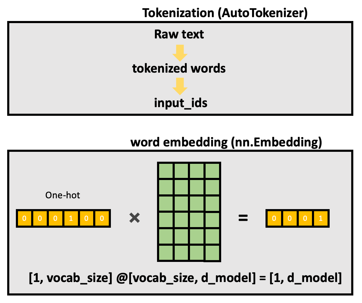
3.1 nn.Embedding
nn.Embedding(vocab_size, d_model) is equivalent to nn.Linear(vocab_size, d_model), offers the [vocab_size, d_model] matrix to multiply.
Class TextEncoder(nn.Module):
	def __init__(self):
		super().__init__()
		self.embed = nn.Embedding(num_embeddings=30522, embedding_dim=512)

	def forward(self, x):
		x = self.embed(x)
		return x

if __name__ == "__main__":
	text_encoder = TextEncoder()
	input = torch.LongTensor([[1, 2, 4, 5], [4, 3, 2, 9]]) # [batch_size, seq_len] = [2, 4]
	hidden_states = text_encoder(x)
	print(hidden_states)
input: [batch_size, seq_len]
hidden states: [batch_size, seq_len, d_model]
For one batch(single sentence),
[seq_len, vocab_size] @ [vocab_size, d_model] = [seq_len, d_model]
For multiple batches(multiple sentences),
[batch_size, seq_len, vocab_size] @ [vocab_size, d_model] = [batch_size, seq_len, d_model]
3.2 nn.Linear
nn.Parameter
self.dense = nn.Linear(in_features=16, out_features=64)

>>m = nn.Linear(20, 30)
>>input = torch.randn(128, 20)
>>output = m(input) # [128,20] @ [20,30] = [128, 30]
>>print(output.size())

m.weight # [out_features, in_features]
4 Training Pipeline
Libraries
import torch
import torch.nn as nn
from torch.optim import SGD, Adagrad, RMSProp, Adam, AdamW
from torch.optim.lr_scheduler import ReduceLROnPlateau
from torch.cuda.amp import GradScaler, autocast
import torch.nn.functional as F
Config
config = {
    "beam_width" : 50,
    "lr"         : 0.01,
    "epochs"     : 1000,
    "batch_size" : 128,
    "input_size" : 13,
    "embed_size" : 896,
    "output_size": len(PHONEMES),
    "momentum"   : 0.9,
    "weight_decay": 1e-5,
    'scheduler_mode' : 'min',  # Assuming you want to minimize a metric like 'val_loss'
    'lr_factor'      : 0.1,    # Factor to reduce the learning rate
    'lr_patience'    : 5,      # Number of epochs with no improvement after which learning rate will be reduced
    'min_lr'         : 1e-9    # Minimum learning rate
}
Training Setup
criterion = nn.CTCLoss(blank=0, reduction='mean', zero_infinity=True)
optimizer = SGD(model.parameters(), lr=config['lr'], momentum=config['momentum'], weight_decay=config['weight_decay'])
# optimizer = AdamW(model.parameters(), lr=0.001, weight_decay=1e-5)
decoder = CTCBeamDecoder(labels=PHONEMES, blank_id=0, beam_width=300, num_processes=4, log_probs_input=True)
scheduler = torch.optim.lr_scheduler.ReduceLROnPlateau(optimizer, mode=config['scheduler_mode'],
                              factor=config['lr_factor'], patience=config['lr_patience'],
                              min_lr=config['min_lr'])
scaler = GradScaler()
5 Criterion
5.1 MSELoss
import torch.nn as nn

criterion = nn.MSELoss()
5.2 CrossEntropyLoss
(1) Information Quantity
The smaller probability, the more Information Quantity
(2) Entropy
The definition of Entropy for a probability distribution is:
\(H(p) = - \sum_{i=1}^{N} p(x_i) \log p(x_i)\)
(3) K-L Divergence(Similarity between the two distributions)
\(D_{KL}(p||q) = \mathbb{E}[\log p(x) - \log q(x)]\)
\(D_{KL}(p||q) = \sum_{i=1}^{N} p(x_i) \log \dfrac{p(x_i)}{q(x_i)}\)
\(D_{KL}(p||q) = H(p,q) - H(p)\)
(4) Cross Entropy
-
Multiclass Classification
\(H(p,q) = - \sum_{i=1}^{N} p(x_i) \log q(x_i) = -\log q(x_+)\)
\(q(i) = softmax(z_i) = \dfrac{e^{z_i}}{\sum e^{z_j}}\) -
Binary Classification
\(H(p,q) = -p \log(q) + (1 - p) \log(1 - q)\) -
Minimum Cross Entropy Loss = Maximum Likelihood Estimation(MLE)
\(arg\) \(min [- \sum p(i) \log q(i)]\) = \(arg\) \(max [ \sum p(i) \log q(i)]\)
In \(softmax\) formula, the probabilty of the true sample(class) through model computes:
In Supervised Learning, Groud Truth is the one-hot vector(for instance: [0,1,0,0], where K=4), So the cross entropy loss:
Example:
Given the Groud-truth values: [1, 0, 0, 0, 0], Prediction values: [0.4, 0.3, 0.05, 0.05, 0.2].
\(\begin{aligned} H(p,q)&= -\sum_i p(i)\log q(i) \\ &= -(1\log0.4 + 0\log0.3 + 0\log0.05 + 0\log0.05 + 0\log0.2) \\ &= -\log0.4 \\ &≈ 0.916 \end{aligned}\)
import torch.nn as nn

criterion = nn.CrossEntropyLoss()
6 Optimizer
Resource 1: 优化器|SGD|Momentum|Adagrad|RMSProp|Adam - Bilibili
Resource 2: AdamW and Adam with weight decay
Resource 3: 非凸函数上,随机梯度下降能否收敛?网友热议:能,但有条件,且比凸函数收敛更难 - 机器之心

梯度下降法有三种不同的形式:
- BGD(Batch Gradient Descent): 批量梯度下降,每次参数更新使用所有样本。
- SGD(Stochastic Gradient Descent): 随机梯度下降,每次参数更新只使用1个样本。
- MBGD(Mini-Batch Gradient Descent): 小批量梯度下降,每次参数更新使用小部分数据样本(mini-batch), 设置超参数batch_size
这三个优化算法在训练的时候虽然所采用的的数据量不同,但是他们在进行参数优化的时候,采用的方法是相同的:
- step 1: $g = \frac{\partial loss}{\partial w} $
- step 2: 求梯度的平均值
- step 3: 更新权重: \(w \leftarrow w - \eta * g\)
(3)优缺点
优点:
。算法简洁,当学习率取值恰当时,可以收敛到 全局最优点(凸函数) 或 局部最优点(非凸函数)。
缺点:
。对超参数学习率比较敏感:过小导致收敛速度过慢,过大又越过极值点
。学习率除了敏感,有时还会因其在迭代过程中保持不变,很容易造成算法被卡在鞍点的位置
。在较平坦的区域,由于梯度接近于0,优化算法会因误判,在还未到达极值点时,就提前结束迭代,陷入局部极小值。
(1)
(2)
(3)
$v_t \gets \beta_1 v_{t-1} +(1-\beta_1)g_{t} $
$r_t \gets \beta_2 r_{t-1} +(1-\beta_2)g^2 $
$\hat{v}_t = \dfrac{v_t}{1-\beta_1}$
$\hat{r}_t = \dfrac{r_t}{1-\beta_2}$
$\theta \gets \theta - \dfrac{\eta}{\sqrt{\hat{r}_t}+\epsilon}*\hat{v}_t $
6.1 SGD with Momentum
optimizer = SGD(
	model.parameters(),
	lr=0.01,
	momentum=0.9)
6.2 Adagrad
optimizer = Adagrad(
	model.parameters(),
	lr=0.01,
	lr_decay=0,
	weight_decay=0,
	initial_accumulator_value=0,
	eps=1e-10
)
6.3 RMSProp
optimizer = RMSProp(
	model.parameters(),
	lr=0.01,
	alpha=0.99,
	eps=1e-08,
	weight_decay=0,
	momentum=0
)
6.4 Adam
optimizer = Adam(
	model.parameters(),
	lr=0.001,
	beta=(0.9,0.999),
	eps=1e-08,
	weight_decay=0
)
6.5 AdamW
optimizer = AdamW(
	model.parameters(),
	lr=0.001,
	betas=(0.9, 0.999),
	eps=1e-08,
	weight_decay=0.01
)
7 Scheduler
Resource 1: 学习率 | warm up 热身训练 | 学习率调度器
8 Scaler
Resource 1: torch.cuda.amp.GradScaler
9 Activation
Blog 1: Activation Functions in Neural Networks [12 Types & Use Cases]
In PyTorch, there are two ways to use the activation functions.
- One is from torch.nn
- First, define
self.softmax = nn.Softmax()indef __init__(self) - Then,
self.softmax(logits)
- First, define
- Another is from torch.nn.functional (
__call__)- Directly,
F.softmax(logits)
- Directly,
9.1 Sigmoid
Sigmoid function is commonly used for the binary classification task, which maps the vector value into (0,1).
import torch.nn.functional as F

scores = F.sigmoid(logits, dim = -1)
from scratch
class Sigmoid:
    def forward(self, Z):
        self.A = 1 / (1 + np.exp(-Z))
        return self.A

    def backward(self, dLdA):
        dAdZ = self.A * (1 - self.A)
        dLdZ = dLdA * dAdZ
        return dLdZ
9.2 Softmax
Softmax function is commonly used for the multiclass classification task, which maps the vector value into (0,1), and return a probability distribution(the sum equals to 1).
For the true class sample,
import torch
import torch.nn.functional as F

with torch.no_grad():
    outputs = model(**batch_input) # SequenceClassifierOutput(loss=None, logits=tensor([[ 0.2347, -0.1015],[ 0.1364, -0.3081],[ 0.0071, -0.4359]], grad_fn=<AddmmBackward0>), hidden_states=None, attentions=None)
    logits = outputs.logits # tensor([[-3.4620,  3.6118],[ 4.7508, -3.7899],[-4.2113,  4.5724]])
    prob_distribution = F.softmax(logits, dim=-1) # tensor([[8.4632e-04, 9.9915e-01],[9.9980e-01, 1.9531e-04],[1.5318e-04, 9.9985e-01]])
    output_ids = torch.argmax(scores, dim=-1) # tensor([1, 0, 1])
    labels = [model.config.id2label[id] for id in output_ids.tolist()] # ['POSITIVE', 'NEGATIVE', 'POSITIVE']
from scratch
class Softmax:
    def forward(self, Z):
        expZ = np.exp(Z - np.max(Z, axis=1, keepdims=True))
        self.A = expZ / np.sum(expZ, axis=1, keepdims=True)
        return self.A

    def backward(self, dLdA):

        # Calculate the batch size and number of features
        N = dLdA.shape[0]
        C = dLdA.shape[1]

        # Initialize the final output dLdZ with all zeros. Refer to the writeup and think about the shape.
        dLdZ = np.zeros_like(dLdA)

        # Fill dLdZ one data point (row) at a time
        for i in range(N):

            # Initialize the Jacobian with all zeros.
            J = np.zeros((C, C))

            # Fill the Jacobian matrix according to the conditions described in the writeup
            for m in range(C):
                for n in range(C):
                    if m == n:
                        J[m,n] = self.A[i, m] * (1 - self.A[i, m])
                    else:
                        J[m, n] = -self.A[i, m] * self.A[i, n]

            # Calculate the derivative of the loss with respect to the i-th input
            dLdZ[i,:] = np.dot(J, dLdA[i, :])

        return dLdZ
9.3 Tanh
Tanh function is commonly used in the Model Head.
import torch.nn as nn
import torch.nn.functional as F

class ModelHead(nn.Module):
    def __init__(self, config):
        self.proj = nn.Linear(config.hidden_size, config.hidden_size)
        self.out_proj = nn.Linear(config.hidden_size, config.num_labels)
    def forward(self, x):
        logits = self.out_proj(F.tanh(self.proj(x), dim = -1))
        prob_distribution = F.softmax(logits, dim=-1)
        output_ids = torch.argmax(prob_distribution, dim=-1)
        labels = [model.config.id2label[id] for id in output_ids.tolist()]
        return labels
9.4 ReLU
ReLU function is used in the feed forward network of the original Transformer(2017) architecture.
import torch.nn as nn
import torch.nn.functional as F

class MLP(nn.Module):
    def __init__(self, config):
        self.up_proj = nn.Linear(config.hidden_size, config.intermediate_size)
        self.down_proj = nn.Linear(config.intermediate_size, config.hidden_size)
    def forward(self, x):
        hidden_states = self.down_proj(F.relu(self.up_proj(x), dim = -1))
        return hidden_states
9.5 SwiGLU
SwiGLU means Swish(also refers to SiLU) and Gated Linear Unit, which is commonly used in the feed forward network of LLaMA 2, Mixtral 7B, Mixtral 8×7B.
import torch.nn as nn
import torch.nn.functional as F

class MLP(nn.Module):
    def __init__(self, config):
        self.up_proj = nn.Linear(config.hidden_size, config.intermediate_size)
        self.gate_proj = nn.Linear(config.hidden_size, config.intermediate_size)
        self.down_proj = nn.Linear(config.intermediate_size, config.hidden_size)
    def forward(self, x):
        hidden_states = self.down_proj(F.silu(self.gate_proj(x), dim = -1) * self.up_proj(x))
        return hidden_states
Reference
Understand collate_fn in PyTorch
【手把手带你实战HuggingFace Transformers-入门篇】基础组件之Model(下)BERT文本分类代码实例

 浙公网安备 33010602011771号