CS231N Assignment4 Two Layer Net
CS231N Assignment4 Two Layer Net
Begin
本文主要介绍CS231N系列课程的第四项作业,写一个两层神经网络训练模型。
课程主页:网易云课堂CS231N系列课程
语言:Python3.6

1神经网络
神经网络理解起来比较简单,在线形分类器的基础上加一个非线性激活函数,使其可以表示非线性含义,再增加
多层分类器就成为多层神经网络,如下图所示,由输入X经过第一层计算得到W1X,在后再用隐含层的激活函数max(0,s)
得到隐含层的输出。到输出层乘以W2得到输出层,最后的分类计分。
下图中最左侧为3072代表每幅图像有3072个特征,经过第一层网络到达中间层叫做隐藏层,隐含层变为100个特征了,在经过第二层计算到输出层最终得到10个类的得分。此神经网络叫做两层的神经网络(包含W1、W2)也叫有一个隐含层的神经网络。
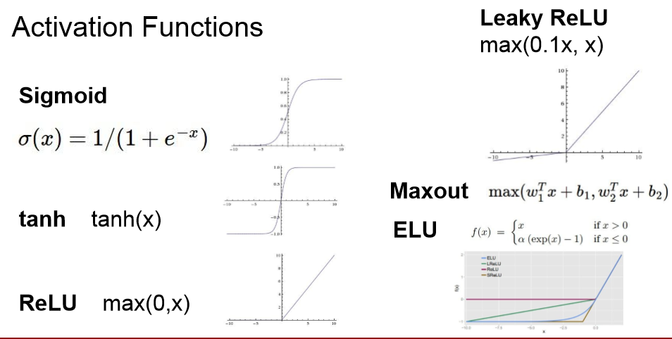
对于激活函数只有在隐含层计算时有激活函数。

对于激活函数,有很多种,如下所示,上述中我们采用的是RELU
2编写一个两层神经网络
类似于之前我们书写的SVM等,编写任何一个训练器需要包含以下几部分
1、LOSS损失函数(前向传播)与梯度(后向传播)计算
2、训练函数
3、预测函数
4、参数训练
2.1 loss函数
损失函数计算采用softmaxu损失方法
1、首先计算前向传输,计算分数,就是上面那三个公式的调用
##############################
        #Computing the class scores of the input
        ##############################
        Z1 = X.dot(W1) + b1#第一层
        S1 = np.maximum(0,Z1)#隐藏层激活函数
        score = S1.dot(W2) + b2#输出层
2、计算完之后,插入一句话,当没有y参数时,直接输出分数,主要用在计算预测函数时需要计算分数。
        if Y is None:
            return score
        loss = None
3、之后计算损失softmax计算,具体计算可以参考我的作业3
        ###############################
        #TODO:forward pass
        #computing the loss of the net
        ################################
        exp_scores = np.exp(score)
        probs = exp_scores / np.sum(exp_scores,axis=1,keepdims=True)
        #数据损失
        data_loss = -1.0/ N * np.log(probs[np.arange(N),Y]).sum()
        #正则损失
        reg_loss = 0.5*reg*(np.sum(W1*W1) + np.sum(W2*W2))
        #总损失
        loss = data_loss + reg_loss
4、计算后向传播梯度
        ################################
        #TODO:backward pass
        #computing the gradient
        ################################
        grads = {}
        dscores = probs
        dscores[np.arange(N),Y] -= 1
        dscores /= N
        #更新W2B2
        grads['W2'] = S1.T.dot(dscores) + reg *W2
        grads['b2'] = np.sum(dscores,axis = 0)

        #第二层

        dhidden = dscores.dot(W2.T)
        dhidden[S1<=0] = 0

        grads['W1'] = X.T.dot(dhidden) + reg *W1
        grads['b1'] = np.sum(dhidden,axis = 0)
代码如下:
def loss(self,X,Y=None,reg=0.0):
        '''
        计算损失函数
        '''
        W1, b1 = self.params['W1'], self.params['b1']
        W2, b2 = self.params['W2'], self.params['b2']
        N, D = X.shape
        ##############################
        #Computing the class scores of the input
        ##############################
        Z1 = X.dot(W1) + b1#第一层
        S1 = np.maximum(0,Z1)#隐藏层激活函数
        score = S1.dot(W2) + b2#输出层

        if Y is None:
            return score
        loss = None
        ###############################
        #TODO:forward pass
        #computing the loss of the net
        ################################
        exp_scores = np.exp(score)
        probs = exp_scores / np.sum(exp_scores,axis=1,keepdims=True)
        #数据损失
        data_loss = -1.0/ N * np.log(probs[np.arange(N),Y]).sum()
        #正则损失
        reg_loss = 0.5*reg*(np.sum(W1*W1) + np.sum(W2*W2))
        #总损失
        loss = data_loss + reg_loss
        ################################
        #TODO:backward pass
        #computing the gradient
        ################################
        grads = {}
        dscores = probs
        dscores[np.arange(N),Y] -= 1
        dscores /= N
        #更新W2B2
        grads['W2'] = S1.T.dot(dscores) + reg *W2
        grads['b2'] = np.sum(dscores,axis = 0)

        #第二层

        dhidden = dscores.dot(W2.T)
        dhidden[S1<=0] = 0

        grads['W1'] = X.T.dot(dhidden) + reg *W1
        grads['b1'] = np.sum(dhidden,axis = 0)

        return loss,grads
2.2 训练函数
训练参数依然是
学习率learning_rate
正则系数reg
训练步数num_iters
每次训练的采样数量batch_size
1、进入循环中,首先采样一定数据,batch_inx = np.random.choice(num_train, batch_size)
代表从0-》num_train中随机产生batch_size 个数,这些数据其实反应这采样样本的索引
值,然后我们用X_batch = X[batch_inx,:]可以获取到该索引所对应的数据
for it in range(num_iters):
            X_batch = None
            y_batch = None

            #########################################################################
            # TODO: Create a random minibatch of training data and labels, storing  #
            # them in X_batch and y_batch respectively.                             #
            #########################################################################
            batch_inx = np.random.choice(num_train, batch_size)
            X_batch = X[batch_inx,:]
            y_batch = y[batch_inx]
2、取样数据后需要计算损失值和梯度。
# Compute loss and gradients using the current minibatch
            loss, grads = self.loss(X_batch, Y=y_batch, reg=reg)
            loss_history.append(loss)
3、计算完损失之后,需要根据梯度值去更新参数W1、W2、b1、b2。
梯度反映着它的最大变化方向,如果梯度是正的表示增长,我们应该反方向去调控,所以在其基础上
减去学习率乘以梯度值。
            #########################################################################
            # TODO: Use the gradients in the grads dictionary to update the         #
            # parameters of the network (stored in the dictionary self.params)      #
            # using stochastic gradient descent. You'll need to use the gradients   #
            # stored in the grads dictionary defined above.                         #
            #########################################################################
            self.params['W1'] -= learning_rate * grads['W1']
            self.params['b1'] -= learning_rate * grads['b1']
            self.params['W2'] -= learning_rate * grads['W2']
            self.params['b2'] -= learning_rate * grads['b2']
4、实时验证
在神经网络训练中我们加入一个实时验证,没训练一次,我们比较以下训练集与预测值的真实程度,
验证集与预测值的真实程度。在最后时可以将这条曲线绘制观测一下。
# Every epoch, check train and val accuracy and decay learning rate.
            if it % iterations_per_epoch == 0:
                # Check accuracy
                train_acc = (self.predict(X_batch) == y_batch).mean()
                val_acc = (self.predict(X_val) == y_val).mean()
                train_acc_history.append(train_acc)
                val_acc_history.append(val_acc)
                # Decay learning rate
                learning_rate *= learning_rate_decay
最终总代码如下所示:
def train(self, X, y, X_val, y_val,
            learning_rate=1e-3, learning_rate_decay=0.95,
            reg=1e-5, num_iters=100,
            batch_size=200, verbose=False):
        """
        Train this neural network using stochastic gradient descent.

        Inputs:
        - X: A numpy array of shape (N, D) giving training data.
        - y: A numpy array f shape (N,) giving training labels; y[i] = c means that
        X[i] has label c, where 0 <= c < C.
        - X_val: A numpy array of shape (N_val, D) giving validation data.
        - y_val: A numpy array of shape (N_val,) giving validation labels.
        - learning_rate: Scalar giving learning rate for optimization.
        - learning_rate_decay: Scalar giving factor used to decay the learning rate
        after each epoch.
        - reg: Scalar giving regularization strength.
        - num_iters: Number of steps to take when optimizing.
        - batch_size: Number of training examples to use per step.
        - verbose: boolean; if true print progress during optimization.
        """
        self.hyper_params = {}
        self.hyper_params['learning_rate'] = learning_rate
        self.hyper_params['reg'] = reg
        self.hyper_params['batch_size'] = batch_size
        self.hyper_params['hidden_size'] = self.params['W1'].shape[1]
        self.hyper_params['num_iter'] = num_iters

        num_train = X.shape[0]
        iterations_per_epoch = max(num_train / batch_size, 1)

        # Use SGD to optimize the parameters in self.model
        loss_history = []
        train_acc_history = []
        val_acc_history = []

        for it in range(num_iters):
            X_batch = None
            y_batch = None

            #########################################################################
            # TODO: Create a random minibatch of training data and labels, storing  #
            # them in X_batch and y_batch respectively.                             #
            #########################################################################
            batch_inx = np.random.choice(num_train, batch_size)
            X_batch = X[batch_inx,:]
            y_batch = y[batch_inx]
            #########################################################################
            #                             END OF YOUR CODE                          #
            #########################################################################

            # Compute loss and gradients using the current minibatch
            loss, grads = self.loss(X_batch, Y=y_batch, reg=reg)
            loss_history.append(loss)

            #########################################################################
            # TODO: Use the gradients in the grads dictionary to update the         #
            # parameters of the network (stored in the dictionary self.params)      #
            # using stochastic gradient descent. You'll need to use the gradients   #
            # stored in the grads dictionary defined above.                         #
            #########################################################################
            self.params['W1'] -= learning_rate * grads['W1']
            self.params['b1'] -= learning_rate * grads['b1']
            self.params['W2'] -= learning_rate * grads['W2']
            self.params['b2'] -= learning_rate * grads['b2']
            #########################################################################
            #                             END OF YOUR CODE                          #
            #########################################################################

            if verbose and it % 100 == 0:
                print ('iteration %d / %d: loss %f' % (it, num_iters, loss))

            # Every epoch, check train and val accuracy and decay learning rate.
            if it % iterations_per_epoch == 0:
                # Check accuracy
                train_acc = (self.predict(X_batch) == y_batch).mean()
                val_acc = (self.predict(X_val) == y_val).mean()
                train_acc_history.append(train_acc)
                val_acc_history.append(val_acc)
                # Decay learning rate
                learning_rate *= learning_rate_decay

        return {
        'loss_history': loss_history,
        'train_acc_history': train_acc_history,
        'val_acc_history': val_acc_history,
        }
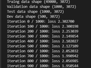
训练时间可能稍微较长,等待一段时间后可以看到如下结果
2.3 predict函数
预测和之前类似,将数据带入损失,找分数最大值即可
def predict(self, X):

        y_pred = None

        scores = self.loss(X)
        y_pred = np.argmax(scores, axis=1)

        return y_pred
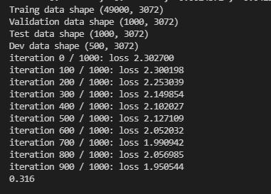
训练结果如下所示
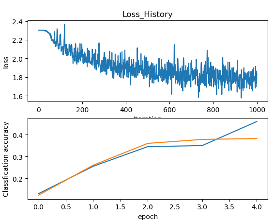
2.4 可视化结果
训练完之后我们可以进行可视化观察,我们把训练时的loss显示出来,还有实时比较的误差拿出来看看。
测试代码如下:
#step1 数据裁剪
#数据量太大,我们重新整理数据,提取一部分训练数据、测试数据、验证数据
num_training = 49000#训练集数量
num_validation = 1000#验证集数量
num_test = 1000#测试集数量
num_dev = 500
Data = load_CIFAR10()
CIFAR10_Data = './'
X_train,Y_train,X_test,Y_test = Data.load_CIFAR10(CIFAR10_Data)#load the data
#从训练集中截取一部分数据作为验证集
mask = range(num_training,num_training + num_validation)
X_val = X_train[mask]
Y_val = Y_train[mask]
#训练集前一部分数据保存为训练集
mask = range(num_training)
X_train = X_train[mask]
Y_train = Y_train[mask]
#训练集数量太大,我们实验只要一部分作为开发集
mask = np.random.choice(num_training,num_dev,replace = False)
X_dev = X_train[mask]
Y_dev = Y_train[mask]
#测试集也太大,变小
mask = range(num_test)
X_test = X_test[mask]
Y_test = Y_test[mask]
#step2 数据预处理
#所有数据准变为二位数据,方便处理
X_train = np.reshape(X_train,(X_train.shape[0],-1))
X_val = np.reshape(X_val,(X_val.shape[0],-1))
X_test = np.reshape(X_test,(X_test.shape[0],-1))
X_dev = np.reshape(X_dev,(X_dev.shape[0],-1))
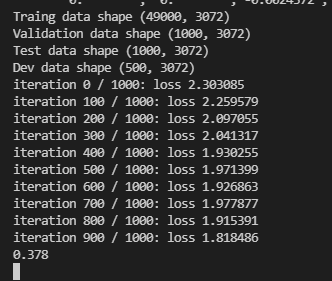
print('Traing data shape', X_train.shape)
print('Validation data shape',X_val.shape)
print('Test data shape',X_test.shape)
print('Dev data shape',X_dev.shape)
#step3训练数据
input_size = 32*32*3
hidden_size = 50
num_classes = 10
net = TwoLayerNet(input_size,hidden_size,num_classes)
#训练
sta = net.train(X_train,Y_train,X_val,Y_val,num_iters=1000,batch_size=200,learning_rate=4e-4,learning_rate_decay=0.95,reg=0.7,verbose=True)
#step4预测数据
val = (net.predict(X_val) == Y_val).mean()
print(val)
#step5可视化效果
plt.subplot(2,1,1)
plt.plot(sta['loss_history'])
plt.ylabel('loss')
plt.xlabel('Iteration')
plt.title('Loss_History')
plt.subplot(2,1,2)
plt.plot(sta['train_acc_history'],label = 'train')
plt.plot(sta['val_acc_history'],label = 'val')
plt.xlabel('epoch')
plt.ylabel('Classfication accuracy')
plt.show()

 浙公网安备 33010602011771号