ANZ Chengdu Data Science Competition

problem requirement

we are provided with a dataset which is related to direct marketing campaigns (phone calls) of a banking institution.
The business problem is to predict whether the client will subscribe to a term deposit.

how to analysis

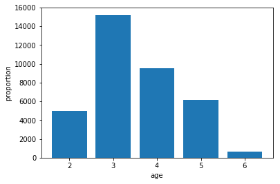
First of all,considering that people of similar age will make an approximate choice, we divide the age by ten.

data['single_year']=data['age']/10
data[['single_year']] = data[['single_year']].astype(int)

Then we draw a histogram of the age to analyze the age distribution in the data.

import matplotlib.pyplot as plt

type_name=data['single_year'].unique()

name_list = type_name
tot=data.count()['y']
num_list = []
dict = {}
for key in data['single_year']:
    dict[key] = dict.get(key, 0) + 1

print(dict)
from matplotlib.font_manager import FontProperties

for key in name_list:
    num_list.append(dict[key])

#print(name_list)
#print(num_list)
propor = num_list

age =type_name


plt.bar(name_list,num_list)

#plt.legend()

plt.xlabel('age')
plt.ylabel('proportion')

#plt.title(u'直方图', FontProperties=font)

plt.show()
del (dict)

It is not difficult to find that the proportion of people over 70 years old is very low.And considering that it is unlikely that older people over the age of 90 will buy products, we decided to screen out data for people over the age of 90.

data.age[(data['age']>=90)|(data['age']<20)]=np.nan
data.dropna(inplace=True)

Then we analyze other features.
We have calculated the Y of different features and made the following decision.
Considering that the diversity of occupations is not conducive to our analysis, we divide the original twelve occupations into four categories.
Changes in one to two months are likely to not affect the results, so we map the months to the first half and the second half.

job_classmap={'admin.':4,'entrepreneur':4,'management':4,'blue-collar':3,'housemaid':3,'services':3,
             'technician':3,'retired':1,'self-employed':1,'student':1,'unemployed':1,'unknown':0}
month_classmap={'may':1,'mar':1,'apr':1,'jun':1,'jul':1,'nov':2,'aug':2,'oct':2,'sep':2,'dec':2}
data['job']=data['job'].map(job_classmap)
data['month']=data['month'].map(month_classmap)

Finally we decided to change all the unknown values to the mode of this feature.

label = data.columns
for i in label:
    if data[i].dtype==data['y'].dtype:
        tmp = data[i].unique()
        print(i,':',tmp)
        tmp.tolist()
        _list=list(range(1,len(tmp)+1))
        classmap=dict(zip(tmp,_list))
        classmap['unknown']=np.NaN
        data[i]=data[i].map(classmap)

For better results, we try to log the logarithm of some continuous variables.

data['log.cons.price.idx']=np.log(data['cons.price.idx'])
data['log.nr.employed']=np.log(data['nr.employed'])

Finally, we tested several models, and finally we used the ‘LogisticRegression’ model based on the accuracy of the prediction.

target = data['y']
del data['duration']
del data['y']
test_data =data[:5000]
data1 = data[5000:10610]
data2 = data[10610:]

target1 = target[5000:10610]
target2 = target[10610:]
del data['age']
mm = MinMaxScaler()
#mean_data
mm_data1=mm.fit_transform(data1)
mm_data2=mm.fit_transform(data2)
# mm_data1=data1;
# mm_data2=data2
lr = LogisticRegression().fit(mm_data1,target1)
lr_ans = lr.predict(mm_data2)
print('lr:',accuracy_score(lr_ans,target2))

svm = SVC(kernel='rbf',C=1.0).fit(mm_data1,target1)
svm_ans = svm.predict(mm_data2)
print('svm:',accuracy_score(svm_ans,target2))

estimator_dt = DecisionTreeClassifier(max_depth=3).fit(mm_data1,target1)
ada = AdaBoostClassifier(estimator_dt,n_estimators=100).fit(mm_data1,target1)
ada_ans = ada.predict(mm.fit_transform(data2))
print('ada:',accuracy_score(ada_ans,target2))

gbdt = GradientBoostingClassifier().fit(mm_data1,target1)
gbdt_ans=gbdt.predict(mm_data2)
print('gbdt:',accuracy_score(gbdt_ans,target2))

lr: 0.899943149517
svm: 0.897858631798
ada: 0.883153306803
gbdt: 0.899147242752