
Python实现随机森林RF并对比自变量的重要性
本文介绍在Python环境中,实现随机森林(Random Forest,RF)回归与各自变量重要性分析与排序的过程。
其中,关于基于MATLAB实现同样过程的代码与实战,大家可以点击查看这篇博客1。
本文分为两部分,第一部分为代码的分段讲解,第二部分为完整代码。
1 代码分段讲解
1.1 模块与数据准备
首先,导入所需要的模块。在这里,需要pydot与graphviz这两个相对不太常用的模块,即使我用了Anaconda,也需要单独下载、安装。具体下载与安装,如果同样是在用Anaconda,大家就参考这篇博客即可。
import pydot
import numpy as np
import pandas as pd
import scipy.stats as stats
import matplotlib.pyplot as plt
from sklearn import metrics
from openpyxl import load_workbook
from sklearn.tree import export_graphviz
from sklearn.ensemble import RandomForestRegressor
接下来,我们将代码接下来需要用的主要变量加以定义。这一部分大家先不用过于在意,浏览一下继续向下看即可;待到对应的变量需要运用时我们自然会理解其具体含义。
train_data_path='G:/CropYield/03_DL/00_Data/AllDataAll_Train.csv'
test_data_path='G:/CropYield/03_DL/00_Data/AllDataAll_Test.csv'
write_excel_path='G:/CropYield/03_DL/05_NewML/ParameterResult_ML.xlsx'
tree_graph_dot_path='G:/CropYield/03_DL/05_NewML/tree.dot'
tree_graph_png_path='G:/CropYield/03_DL/05_NewML/tree.png'

random_seed=44
random_forest_seed=np.random.randint(low=1,high=230)
接下来,我们需要导入输入数据。
在这里需要注意,本文对以下两个数据处理的流程并没有详细涉及与讲解(因为在写本文时,我已经做过了同一批数据的深度学习回归,本文就直接用了当时做深度学习时处理好的输入数据,因此以下两个数据处理的基本过程就没有再涉及啦),大家直接查看下方所列出的其它几篇博客即可。
-
初始数据划分训练集与测试集
-
类别变量的独热编码(One-hot Encoding)
针对上述两个数据处理过程,首先,数据训练集与测试集的划分在机器学习、深度学习中是不可或缺的作用,这一部分大家可以查看这篇博客2的2.4部分,或这篇博客3的2.3部分;其次,关于类别变量的独热编码,对于随机森林等传统机器学习方法而言可以说同样是非常重要的,这一部分大家可以查看这篇博客4。
在本文中,如前所述,我们直接将已经存在.csv中,已经划分好训练集与测试集且已经对类别变量做好了独热编码之后的数据加以导入。在这里,我所导入的数据第一行是表头,即每一列的名称。关于.csv数据导入的代码详解,大家可以查看这篇博客5的数据导入部分。
# Data import

'''
column_name=['EVI0610','EVI0626','EVI0712','EVI0728','EVI0813','EVI0829','EVI0914','EVI0930','EVI1016',
             'Lrad06','Lrad07','Lrad08','Lrad09','Lrad10',
             'Prec06','Prec07','Prec08','Prec09','Prec10',
             'Pres06','Pres07','Pres08','Pres09','Pres10',
             'SIF161','SIF177','SIF193','SIF209','SIF225','SIF241','SIF257','SIF273','SIF289',
             'Shum06','Shum07','Shum08','Shum09','Shum10',
             'Srad06','Srad07','Srad08','Srad09','Srad10',
             'Temp06','Temp07','Temp08','Temp09','Temp10',
             'Wind06','Wind07','Wind08','Wind09','Wind10',
             'Yield']
'''
train_data=pd.read_csv(train_data_path,header=0)
test_data=pd.read_csv(test_data_path,header=0)
1.2 特征与标签分离
特征与标签,换句话说其实就是自变量与因变量。我们要将训练集与测试集中对应的特征与标签分别分离开来。
# Separate independent and dependent variables

train_Y=np.array(train_data['Yield'])
train_X=train_data.drop(['ID','Yield'],axis=1)
train_X_column_name=list(train_X.columns)
train_X=np.array(train_X)

test_Y=np.array(test_data['Yield'])
test_X=test_data.drop(['ID','Yield'],axis=1)
test_X=np.array(test_X)
可以看到,直接借助drop就可以将标签'Yield'从原始的数据中剔除(同时还剔除了一个'ID',这个是初始数据的样本编号,后面就没什么用了,因此随着标签一起剔除)。同时在这里,还借助了train_X_column_name这一变量,将每一个特征值列所对应的标题(也就是特征的名称)加以保存,供后续使用。
1.3 RF模型构建、训练与预测
接下来,我们就需要对随机森林模型加以建立,并训练模型,最后再利用测试集加以预测。在这里需要注意,关于随机森林的几个重要超参数(例如下方的n_estimators)都是需要不断尝试找到最优的。关于这些超参数的寻优,在MATLAB中的实现方法大家可以查看这篇博客1的1.1部分;而在Python中的实现方法,大家查看这篇博客6即可。
# Build RF regression model

random_forest_model=RandomForestRegressor(n_estimators=200,random_state=random_forest_seed)
random_forest_model.fit(train_X,train_Y)

# Predict test set data

random_forest_predict=random_forest_model.predict(test_X)
random_forest_error=random_forest_predict-test_Y
其中,利用RandomForestRegressor进行模型的构建,n_estimators就是树的个数,random_state是每一个树利用Bagging策略中的Bootstrap进行抽样(即有放回的袋外随机抽样)时,随机选取样本的随机数种子;fit进行模型的训练,predict进行模型的预测,最后一句就是计算预测的误差。
1.4 预测图像绘制、精度衡量指标计算与保存
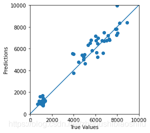
首先,进行预测图像绘制,其中包括预测结果的拟合图与误差分布直方图。关于这一部分代码的解释,大家可以查看这篇博客2的2.9部分。
# Draw test plot

plt.figure(1)
plt.clf()
ax=plt.axes(aspect='equal')
plt.scatter(test_Y,random_forest_predict)
plt.xlabel('True Values')
plt.ylabel('Predictions')
Lims=[0,10000]
plt.xlim(Lims)
plt.ylim(Lims)
plt.plot(Lims,Lims)
plt.grid(False)

plt.figure(2)
plt.clf()
plt.hist(random_forest_error,bins=30)
plt.xlabel('Prediction Error')
plt.ylabel('Count')
plt.grid(False)
以上两幅图的绘图结果如下所示。

接下来,进行精度衡量指标的计算与保存。在这里,我们用皮尔逊相关系数、决定系数与RMSE作为精度的衡量指标,并将每一次模型运行的精度衡量指标结果保存在一个Excel文件中。这一部分大家同样查看这篇博客2的2.9部分即可。
# Verify the accuracy

random_forest_pearson_r=stats.pearsonr(test_Y,random_forest_predict)
random_forest_R2=metrics.r2_score(test_Y,random_forest_predict)
random_forest_RMSE=metrics.mean_squared_error(test_Y,random_forest_predict)**0.5
print('Pearson correlation coefficient is {0}, and RMSE is {1}.'.format(random_forest_pearson_r[0],
                                                                        random_forest_RMSE))

# Save key parameters

excel_file=load_workbook(write_excel_path)
excel_all_sheet=excel_file.sheetnames
excel_write_sheet=excel_file[excel_all_sheet[0]]
excel_write_sheet=excel_file.active
max_row=excel_write_sheet.max_row
excel_write_content=[random_forest_pearson_r[0],random_forest_R2,random_forest_RMSE,random_seed,random_forest_seed]
for i in range(len(excel_write_content)):
        exec("excel_write_sheet.cell(max_row+1,i+1).value=excel_write_content[i]")
excel_file.save(write_excel_path)
1.5 决策树可视化
这一部分我们借助DOT这一图像描述语言,进行随机森林算法中决策树的绘制。
# Draw decision tree visualizing plot

random_forest_tree=random_forest_model.estimators_[5]
export_graphviz(random_forest_tree,out_file=tree_graph_dot_path,
                feature_names=train_X_column_name,rounded=True,precision=1)
(random_forest_graph,)=pydot.graph_from_dot_file(tree_graph_dot_path)
random_forest_graph.write_png(tree_graph_png_path)
其中,estimators_[5]是指整个随机森林算法中的第6棵树(下标是从0开始的),换句话说我们就是从很多的树(具体树的个数就是前面提到的超参数n_estimators)中抽取了找一个来画图,做一个示范。如下图所示。
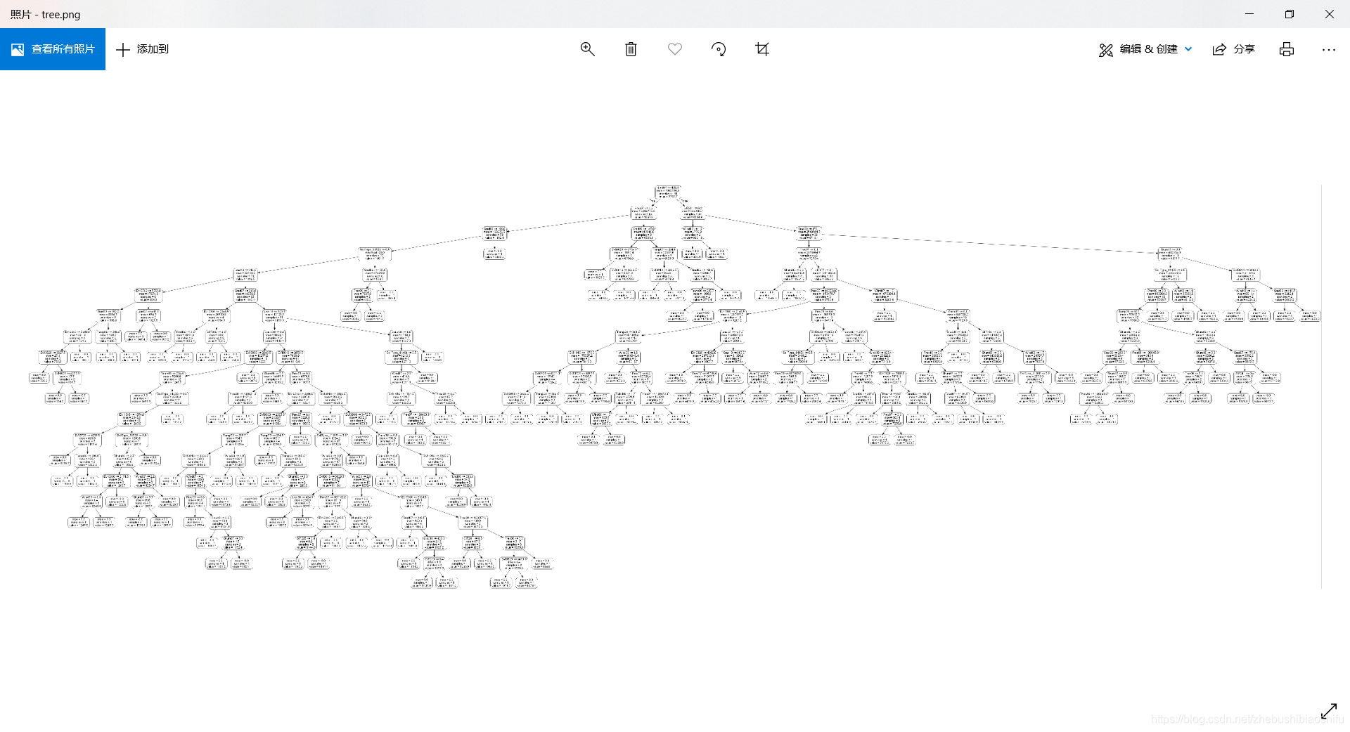
可以看到,单单是这一棵树就已经非常非常庞大了。我们将上图其中最顶端(也就是最上方的节点——根节点)部分放大,就可以看见每一个节点对应的信息。如下图

在这里提一句,上图根节点中有一个samples=151,但是我的样本总数是315个,为什么这棵树的样本个数不是全部的样本个数呢?
其实这就是随机森林的内涵所在:随机森林的每一棵树的输入数据(也就是该棵树的根节点中的数据),都是随机选取的(也就是上面我们说的利用Bagging策略中的Bootstrap进行随机抽样),最后再将每一棵树的结果聚合起来(聚合这个过程就是Aggregation,我们常说的Bagging其实就是Bootstrap与Aggregation的合称),形成随机森林算法最终的结果。
1.6 变量重要性分析
在这里,我们进行变量重要性的分析,并以图的形式进行可视化。
# Calculate the importance of variables

random_forest_importance=list(random_forest_model.feature_importances_)
random_forest_feature_importance=[(feature,round(importance,8))
                                  for feature, importance in zip(train_X_column_name,random_forest_importance)]
random_forest_feature_importance=sorted(random_forest_feature_importance,key=lambda x:x[1],reverse=True)
plt.figure(3)
plt.clf()
importance_plot_x_values=list(range(len(random_forest_importance)))
plt.bar(importance_plot_x_values,random_forest_importance,orientation='vertical')
plt.xticks(importance_plot_x_values,train_X_column_name,rotation='vertical')
plt.xlabel('Variable')
plt.ylabel('Importance')
plt.title('Variable Importances')
得到图像如下所示。这里是由于我的特征数量(自变量数量)过多,大概有150多个,导致横坐标的标签(也就是自变量的名称)都重叠了;大家一般的自变量个数都不会太多,就不会有问题~

以上就是全部的代码分段介绍~
2 完整代码
# -*- coding: utf-8 -*-
"""
Created on Sun Mar 21 22:05:37 2021

@author: fkxxgis
"""

import pydot
import numpy as np
import pandas as pd
import scipy.stats as stats
import matplotlib.pyplot as plt
from sklearn import metrics
from openpyxl import load_workbook
from sklearn.tree import export_graphviz
from sklearn.ensemble import RandomForestRegressor


# Attention! Data Partition
# Attention! One-Hot Encoding

train_data_path='G:/CropYield/03_DL/00_Data/AllDataAll_Train.csv'
test_data_path='G:/CropYield/03_DL/00_Data/AllDataAll_Test.csv'
write_excel_path='G:/CropYield/03_DL/05_NewML/ParameterResult_ML.xlsx'
tree_graph_dot_path='G:/CropYield/03_DL/05_NewML/tree.dot'
tree_graph_png_path='G:/CropYield/03_DL/05_NewML/tree.png'

random_seed=44
random_forest_seed=np.random.randint(low=1,high=230)

# Data import

'''
column_name=['EVI0610','EVI0626','EVI0712','EVI0728','EVI0813','EVI0829','EVI0914','EVI0930','EVI1016',
             'Lrad06','Lrad07','Lrad08','Lrad09','Lrad10',
             'Prec06','Prec07','Prec08','Prec09','Prec10',
             'Pres06','Pres07','Pres08','Pres09','Pres10',
             'SIF161','SIF177','SIF193','SIF209','SIF225','SIF241','SIF257','SIF273','SIF289',
             'Shum06','Shum07','Shum08','Shum09','Shum10',
             'Srad06','Srad07','Srad08','Srad09','Srad10',
             'Temp06','Temp07','Temp08','Temp09','Temp10',
             'Wind06','Wind07','Wind08','Wind09','Wind10',
             'Yield']
'''
train_data=pd.read_csv(train_data_path,header=0)
test_data=pd.read_csv(test_data_path,header=0)

# Separate independent and dependent variables

train_Y=np.array(train_data['Yield'])
train_X=train_data.drop(['ID','Yield'],axis=1)
train_X_column_name=list(train_X.columns)
train_X=np.array(train_X)

test_Y=np.array(test_data['Yield'])
test_X=test_data.drop(['ID','Yield'],axis=1)
test_X=np.array(test_X)

# Build RF regression model

random_forest_model=RandomForestRegressor(n_estimators=200,random_state=random_forest_seed)
random_forest_model.fit(train_X,train_Y)

# Predict test set data

random_forest_predict=random_forest_model.predict(test_X)
random_forest_error=random_forest_predict-test_Y

# Draw test plot

plt.figure(1)
plt.clf()
ax=plt.axes(aspect='equal')
plt.scatter(test_Y,random_forest_predict)
plt.xlabel('True Values')
plt.ylabel('Predictions')
Lims=[0,10000]
plt.xlim(Lims)
plt.ylim(Lims)
plt.plot(Lims,Lims)
plt.grid(False)

plt.figure(2)
plt.clf()
plt.hist(random_forest_error,bins=30)
plt.xlabel('Prediction Error')
plt.ylabel('Count')
plt.grid(False)

# Verify the accuracy

random_forest_pearson_r=stats.pearsonr(test_Y,random_forest_predict)
random_forest_R2=metrics.r2_score(test_Y,random_forest_predict)
random_forest_RMSE=metrics.mean_squared_error(test_Y,random_forest_predict)**0.5
print('Pearson correlation coefficient is {0}, and RMSE is {1}.'.format(random_forest_pearson_r[0],
                                                                        random_forest_RMSE))

# Save key parameters

excel_file=load_workbook(write_excel_path)
excel_all_sheet=excel_file.sheetnames
excel_write_sheet=excel_file[excel_all_sheet[0]]
excel_write_sheet=excel_file.active
max_row=excel_write_sheet.max_row
excel_write_content=[random_forest_pearson_r[0],random_forest_R2,random_forest_RMSE,random_seed,random_forest_seed]
for i in range(len(excel_write_content)):
        exec("excel_write_sheet.cell(max_row+1,i+1).value=excel_write_content[i]")
excel_file.save(write_excel_path)

# Draw decision tree visualizing plot

random_forest_tree=random_forest_model.estimators_[5]
export_graphviz(random_forest_tree,out_file=tree_graph_dot_path,
                feature_names=train_X_column_name,rounded=True,precision=1)
(random_forest_graph,)=pydot.graph_from_dot_file(tree_graph_dot_path)
random_forest_graph.write_png(tree_graph_png_path)

# Calculate the importance of variables

random_forest_importance=list(random_forest_model.feature_importances_)
random_forest_feature_importance=[(feature,round(importance,8))
                                  for feature, importance in zip(train_X_column_name,random_forest_importance)]
random_forest_feature_importance=sorted(random_forest_feature_importance,key=lambda x:x[1],reverse=True)
plt.figure(3)
plt.clf()
importance_plot_x_values=list(range(len(random_forest_importance)))
plt.bar(importance_plot_x_values,random_forest_importance,orientation='vertical')
plt.xticks(importance_plot_x_values,train_X_column_name,rotation='vertical')
plt.xlabel('Variable')
plt.ylabel('Importance')
plt.title('Variable Importances')
至此,大功告成。

 浙公网安备 33010602011771号