9,K-近邻算法(KNN)
导引:
如何进行电影分类
众所周知,电影可以按照题材分类,然而题材本身是如何定义的?由谁来判定某部电影属于哪 个题材?也就是说同一题材的电影具有哪些公共特征?这些都是在进行电影分类时必须要考虑的问 题。没有哪个电影人会说自己制作的电影和以前的某部电影类似,但我们确实知道每部电影在风格 上的确有可能会和同题材的电影相近。那么动作片具有哪些共有特征,使得动作片之间非常类似, 而与爱情片存在着明显的差别呢?动作片中也会存在接吻镜头,爱情片中也会存在打斗场景,我们 不能单纯依靠是否存在打斗或者亲吻来判断影片的类型。但是爱情片中的亲吻镜头更多,动作片中 的打斗场景也更频繁,基于此类场景在某部电影中出现的次数可以用来进行电影分类。
本章介绍第一个机器学习算法:K-近邻算法,它非常有效而且易于掌握。
1、k-近邻算法原理
简单地说,K-近邻算法采用测量不同特征值之间的距离方法进行分类。
- 优点:精度高(计算距离)、对异常值不敏感(单纯根据距离进行分类,会忽略特殊情况)、无数据输入假定(不会对数据预先进行判定)。
- 缺点:时间复杂度高、空间复杂度高。
- 适用数据范围:数值型和标称型。
工作原理
存在一个样本数据集合,也称作训练样本集,并且样本集中每个数据都存在标签,即我们知道样本集中每一数据 与所属分类的对应关系。输人没有标签的新数据后,将新数据的每个特征与样本集中数据对应的 特征进行比较,然后算法提取样本集中特征最相似数据(最近邻)的分类标签。一般来说,我们 只选择样本数据集中前K个最相似的数据,这就是K-近邻算法中K的出处,通常K是不大于20的整数。 最后 ,选择K个最相似数据中出现次数最多的分类,作为新数据的分类。
回到前面电影分类的例子,使用K-近邻算法分类爱情片和动作片。有人曾经统计过很多电影的打斗镜头和接吻镜头,下图显示了6部电影的打斗和接吻次数。假如有一部未看过的电影,如何确定它是爱情片还是动作片呢?我们可以使用K-近邻算法来解决这个问题。

首先我们需要知道这个未知电影存在多少个打斗镜头和接吻镜头,上图中问号位置是该未知电影出现的镜头数图形化展示,具体数字参见下表。

即使不知道未知电影属于哪种类型,我们也可以通过某种方法计算出来。首先计算未知电影与样本集中其他电影的距离,如图所示。

现在我们得到了样本集中所有电影与未知电影的距离,按照距离递增排序,可以找到K个距 离最近的电影。假定k=3,则三个最靠近的电影依次是California Man、He's Not Really into Dudes、Beautiful Woman。K-近邻算法按照距离最近的三部电影的类型,决定未知电影的类型,而这三部电影全是爱情片,因此我们判定未知电影是爱情片。
欧几里得距离(Euclidean Distance)
欧氏距离是最常见的距离度量,衡量的是多维空间中各个点之间的绝对距离。公式如下:

2、在scikit-learn库中使用k-近邻算法
- 分类问题:from sklearn.neighbors import KNeighborsClassifier
Type Markdown and LaTeX: α2α2
0)一个最简单的例子
身高、体重、鞋子尺码数据对应性别
import numpy as np
import pandas  as pd
from pandas import DataFrame,Series

feature = np.array([[170,75,41],[166,65,38],[177,80,43],[179,80,43],[170,60,40],[160,55,38]])
target = np.array(['男','女','男','男','女','女'])

from sklearn.neighbors import KNeighborsClassifier
knn = KNeighborsClassifier(n_neighbors=3)

knn.fit(feature,target)
knn.score(feature,target)  #1.0

knn.predict(np.array([[176,71,38]]))
# array(['男'], dtype='<U1')
查看电影属于那个类别
df = pd.read_excel('../../my_films.xlsx')
df

feature = df[['Action lens','Love lens']]
target = df['target']

knn = KNeighborsClassifier(n_neighbors=4)
knn.fit(feature,target)
knn.score(feature,target)  #1.0
knn.predict(np.array([[60,42]]))
# array(['Action'], dtype=object)
1)用于分类
数据蓝蝴蝶以及k值的算法
import sklearn.datasets as datasets
iris = datasets.load_iris()
iris


{'data': array([[5.1, 3.5, 1.4, 0.2],
        [4.9, 3. , 1.4, 0.2],
        [4.7, 3.2, 1.3, 0.2],
        [4.6, 3.1, 1.5, 0.2],
        [5. , 3.6, 1.4, 0.2],
        [5.4, 3.9, 1.7, 0.4],
        [4.6, 3.4, 1.4, 0.3],
        [5. , 3.4, 1.5, 0.2],
        [4.4, 2.9, 1.4, 0.2],
        [4.9, 3.1, 1.5, 0.1],
        [5.4, 3.7, 1.5, 0.2],
        [4.8, 3.4, 1.6, 0.2],
        [4.8, 3. , 1.4, 0.1],
        [4.3, 3. , 1.1, 0.1],
        [5.8, 4. , 1.2, 0.2],
        [5.7, 4.4, 1.5, 0.4],
        [5.4, 3.9, 1.3, 0.4],
        [5.1, 3.5, 1.4, 0.3],
        [5.7, 3.8, 1.7, 0.3],
        [5.1, 3.8, 1.5, 0.3],
        [5.4, 3.4, 1.7, 0.2],
        [5.1, 3.7, 1.5, 0.4],
        [4.6, 3.6, 1. , 0.2],
        [5.1, 3.3, 1.7, 0.5],
        [4.8, 3.4, 1.9, 0.2],
        [5. , 3. , 1.6, 0.2],
        [5. , 3.4, 1.6, 0.4],
        [5.2, 3.5, 1.5, 0.2],
        [5.2, 3.4, 1.4, 0.2],
        [4.7, 3.2, 1.6, 0.2],
        [4.8, 3.1, 1.6, 0.2],
        [5.4, 3.4, 1.5, 0.4],
        [5.2, 4.1, 1.5, 0.1],
        [5.5, 4.2, 1.4, 0.2],
        [4.9, 3.1, 1.5, 0.1],
        [5. , 3.2, 1.2, 0.2],
        [5.5, 3.5, 1.3, 0.2],
        [4.9, 3.1, 1.5, 0.1],
        [4.4, 3. , 1.3, 0.2],
        [5.1, 3.4, 1.5, 0.2],
        [5. , 3.5, 1.3, 0.3],
        [4.5, 2.3, 1.3, 0.3],
        [4.4, 3.2, 1.3, 0.2],
        [5. , 3.5, 1.6, 0.6],
        [5.1, 3.8, 1.9, 0.4],
        [4.8, 3. , 1.4, 0.3],
        [5.1, 3.8, 1.6, 0.2],
        [4.6, 3.2, 1.4, 0.2],
        [5.3, 3.7, 1.5, 0.2],
        [5. , 3.3, 1.4, 0.2],
        [7. , 3.2, 4.7, 1.4],
        [6.4, 3.2, 4.5, 1.5],
        [6.9, 3.1, 4.9, 1.5],
        [5.5, 2.3, 4. , 1.3],
        [6.5, 2.8, 4.6, 1.5],
        [5.7, 2.8, 4.5, 1.3],
        [6.3, 3.3, 4.7, 1.6],
        [4.9, 2.4, 3.3, 1. ],
        [6.6, 2.9, 4.6, 1.3],
        [5.2, 2.7, 3.9, 1.4],
        [5. , 2. , 3.5, 1. ],
        [5.9, 3. , 4.2, 1.5],
        [6. , 2.2, 4. , 1. ],
        [6.1, 2.9, 4.7, 1.4],
        [5.6, 2.9, 3.6, 1.3],
        [6.7, 3.1, 4.4, 1.4],
        [5.6, 3. , 4.5, 1.5],
        [5.8, 2.7, 4.1, 1. ],
        [6.2, 2.2, 4.5, 1.5],
        [5.6, 2.5, 3.9, 1.1],
        [5.9, 3.2, 4.8, 1.8],
        [6.1, 2.8, 4. , 1.3],
        [6.3, 2.5, 4.9, 1.5],
        [6.1, 2.8, 4.7, 1.2],
        [6.4, 2.9, 4.3, 1.3],
        [6.6, 3. , 4.4, 1.4],
        [6.8, 2.8, 4.8, 1.4],
        [6.7, 3. , 5. , 1.7],
        [6. , 2.9, 4.5, 1.5],
        [5.7, 2.6, 3.5, 1. ],
        [5.5, 2.4, 3.8, 1.1],
        [5.5, 2.4, 3.7, 1. ],
        [5.8, 2.7, 3.9, 1.2],
        [6. , 2.7, 5.1, 1.6],
        [5.4, 3. , 4.5, 1.5],
        [6. , 3.4, 4.5, 1.6],
        [6.7, 3.1, 4.7, 1.5],
        [6.3, 2.3, 4.4, 1.3],
        [5.6, 3. , 4.1, 1.3],
        [5.5, 2.5, 4. , 1.3],
        [5.5, 2.6, 4.4, 1.2],
        [6.1, 3. , 4.6, 1.4],
        [5.8, 2.6, 4. , 1.2],
        [5. , 2.3, 3.3, 1. ],
        [5.6, 2.7, 4.2, 1.3],
        [5.7, 3. , 4.2, 1.2],
        [5.7, 2.9, 4.2, 1.3],
        [6.2, 2.9, 4.3, 1.3],
        [5.1, 2.5, 3. , 1.1],
        [5.7, 2.8, 4.1, 1.3],
        [6.3, 3.3, 6. , 2.5],
        [5.8, 2.7, 5.1, 1.9],
        [7.1, 3. , 5.9, 2.1],
        [6.3, 2.9, 5.6, 1.8],
        [6.5, 3. , 5.8, 2.2],
        [7.6, 3. , 6.6, 2.1],
        [4.9, 2.5, 4.5, 1.7],
        [7.3, 2.9, 6.3, 1.8],
        [6.7, 2.5, 5.8, 1.8],
        [7.2, 3.6, 6.1, 2.5],
        [6.5, 3.2, 5.1, 2. ],
        [6.4, 2.7, 5.3, 1.9],
        [6.8, 3. , 5.5, 2.1],
        [5.7, 2.5, 5. , 2. ],
        [5.8, 2.8, 5.1, 2.4],
        [6.4, 3.2, 5.3, 2.3],
        [6.5, 3. , 5.5, 1.8],
        [7.7, 3.8, 6.7, 2.2],
        [7.7, 2.6, 6.9, 2.3],
        [6. , 2.2, 5. , 1.5],
        [6.9, 3.2, 5.7, 2.3],
        [5.6, 2.8, 4.9, 2. ],
        [7.7, 2.8, 6.7, 2. ],
        [6.3, 2.7, 4.9, 1.8],
        [6.7, 3.3, 5.7, 2.1],
        [7.2, 3.2, 6. , 1.8],
        [6.2, 2.8, 4.8, 1.8],
        [6.1, 3. , 4.9, 1.8],
        [6.4, 2.8, 5.6, 2.1],
        [7.2, 3. , 5.8, 1.6],
        [7.4, 2.8, 6.1, 1.9],
        [7.9, 3.8, 6.4, 2. ],
        [6.4, 2.8, 5.6, 2.2],
        [6.3, 2.8, 5.1, 1.5],
        [6.1, 2.6, 5.6, 1.4],
        [7.7, 3. , 6.1, 2.3],
        [6.3, 3.4, 5.6, 2.4],
        [6.4, 3.1, 5.5, 1.8],
        [6. , 3. , 4.8, 1.8],
        [6.9, 3.1, 5.4, 2.1],
        [6.7, 3.1, 5.6, 2.4],
        [6.9, 3.1, 5.1, 2.3],
        [5.8, 2.7, 5.1, 1.9],
        [6.8, 3.2, 5.9, 2.3],
        [6.7, 3.3, 5.7, 2.5],
        [6.7, 3. , 5.2, 2.3],
        [6.3, 2.5, 5. , 1.9],
        [6.5, 3. , 5.2, 2. ],
        [6.2, 3.4, 5.4, 2.3],
        [5.9, 3. , 5.1, 1.8]]),
 'target': array([0, 0, 0, 0, 0, 0, 0, 0, 0, 0, 0, 0, 0, 0, 0, 0, 0, 0, 0, 0, 0, 0,
        0, 0, 0, 0, 0, 0, 0, 0, 0, 0, 0, 0, 0, 0, 0, 0, 0, 0, 0, 0, 0, 0,
        0, 0, 0, 0, 0, 0, 1, 1, 1, 1, 1, 1, 1, 1, 1, 1, 1, 1, 1, 1, 1, 1,
        1, 1, 1, 1, 1, 1, 1, 1, 1, 1, 1, 1, 1, 1, 1, 1, 1, 1, 1, 1, 1, 1,
        1, 1, 1, 1, 1, 1, 1, 1, 1, 1, 1, 1, 2, 2, 2, 2, 2, 2, 2, 2, 2, 2,
        2, 2, 2, 2, 2, 2, 2, 2, 2, 2, 2, 2, 2, 2, 2, 2, 2, 2, 2, 2, 2, 2,
        2, 2, 2, 2, 2, 2, 2, 2, 2, 2, 2, 2, 2, 2, 2, 2, 2, 2]),
 'target_names': array(['setosa', 'versicolor', 'virginica'], dtype='<U10'),
 'DESCR': 'Iris Plants Database\n====================\n\nNotes\n-----\nData Set Characteristics:\n    :Number of Instances: 150 (50 in each of three classes)\n    :Number of Attributes: 4 numeric, predictive attributes and the class\n    :Attribute Information:\n        - sepal length in cm\n        - sepal width in cm\n        - petal length in cm\n        - petal width in cm\n        - class:\n                - Iris-Setosa\n                - Iris-Versicolour\n                - Iris-Virginica\n    :Summary Statistics:\n\n    ============== ==== ==== ======= ===== ====================\n                    Min  Max   Mean    SD   Class Correlation\n    ============== ==== ==== ======= ===== ====================\n    sepal length:   4.3  7.9   5.84   0.83    0.7826\n    sepal width:    2.0  4.4   3.05   0.43   -0.4194\n    petal length:   1.0  6.9   3.76   1.76    0.9490  (high!)\n    petal width:    0.1  2.5   1.20  0.76     0.9565  (high!)\n    ============== ==== ==== ======= ===== ====================\n\n    :Missing Attribute Values: None\n    :Class Distribution: 33.3% for each of 3 classes.\n    :Creator: R.A. Fisher\n    :Donor: Michael Marshall (MARSHALL%PLU@io.arc.nasa.gov)\n    :Date: July, 1988\n\nThis is a copy of UCI ML iris datasets.\nhttp://archive.ics.uci.edu/ml/datasets/Iris\n\nThe famous Iris database, first used by Sir R.A Fisher\n\nThis is perhaps the best known database to be found in the\npattern recognition literature.  Fisher\'s paper is a classic in the field and\nis referenced frequently to this day.  (See Duda & Hart, for example.)  The\ndata set contains 3 classes of 50 instances each, where each class refers to a\ntype of iris plant.  One class is linearly separable from the other 2; the\nlatter are NOT linearly separable from each other.\n\nReferences\n----------\n   - Fisher,R.A. "The use of multiple measurements in taxonomic problems"\n     Annual Eugenics, 7, Part II, 179-188 (1936); also in "Contributions to\n     Mathematical Statistics" (John Wiley, NY, 1950).\n   - Duda,R.O., & Hart,P.E. (1973) Pattern Classification and Scene Analysis.\n     (Q327.D83) John Wiley & Sons.  ISBN 0-471-22361-1.  See page 218.\n   - Dasarathy, B.V. (1980) "Nosing Around the Neighborhood: A New System\n     Structure and Classification Rule for Recognition in Partially Exposed\n     Environments".  IEEE Transactions on Pattern Analysis and Machine\n     Intelligence, Vol. PAMI-2, No. 1, 67-71.\n   - Gates, G.W. (1972) "The Reduced Nearest Neighbor Rule".  IEEE Transactions\n     on Information Theory, May 1972, 431-433.\n   - See also: 1988 MLC Proceedings, 54-64.  Cheeseman et al"s AUTOCLASS II\n     conceptual clustering system finds 3 classes in the data.\n   - Many, many more ...\n',
 'feature_names': ['sepal length (cm)',
  'sepal width (cm)',
  'petal length (cm)',
  'petal width (cm)']}
#提取样本数据
feature = iris['data']
target = iris['target']

#将样本数据进行随机打乱
np.random.seed(1)
np.random.shuffle(feature)
np.random.seed(1)
np.random.shuffle(target)

feature.shape #(150, 4)

#获取训练样本数据和测试样本数据
#训练数据
x_train = feature[:140]
y_train = target[:140]
#测试数据
x_test = feature[-10:]
y_test =target[-10:]

#实例化模型对象&训练模型
knn = KNeighborsClassifier(n_neighbors=10)
knn.fit(x_train,y_train)
knn.score(x_train,y_train)   #0.9857142857142858

print('预测分类:',knn.predict(x_test))
print('真实分类:',y_test)
预测分类: [0 2 1 2 0 1 2 1 1 0]
真实分类: [0 2 1 1 0 1 2 1 1 0]
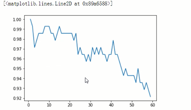
# 选中最优的k值
k_list = []
s_list = []

for k in range(1,60):
    knn = KNeighborsClassifier(n_neighbors=k)
    knn.fit(x_train,y_train)
    s_list.append(s)
    k_list.append(k)

import matplot.pyplot as plt
plt.plot(k_list,s_list)

 浙公网安备 33010602011771号