机器学习【七】神经网络
本章重点介绍“多层感知器”,即MLP算法
MLP也称为前馈神经网络,泛称为神经网络
原理


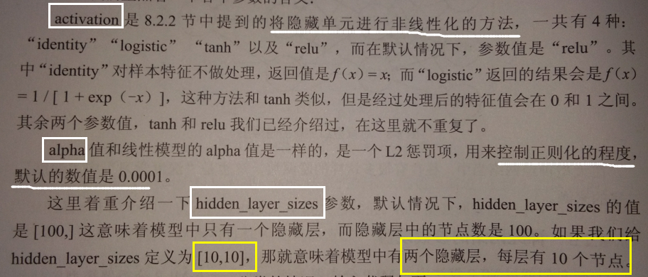
神经网络中的非线性矫正
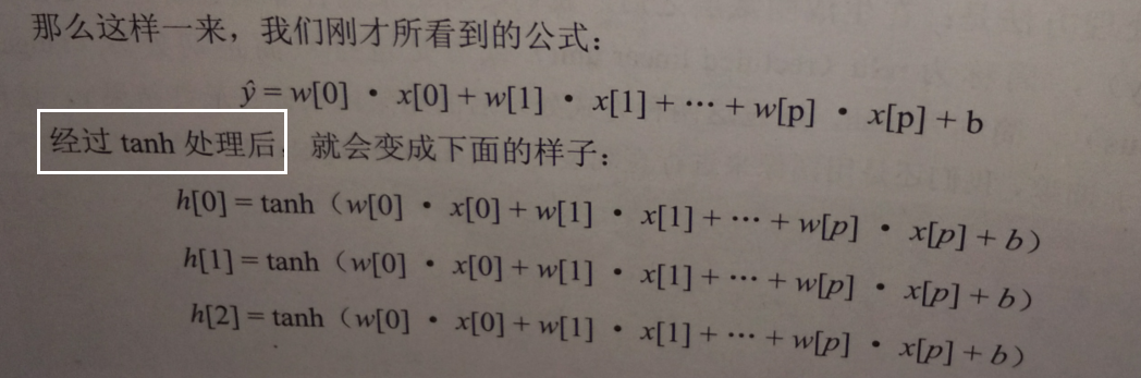
在生成隐藏层后,对 结果进行非线性矫正 rele 或进行双曲正切处理 tanh
通过这两种方式处理后的结果用来计算最终结果y
用图像展示:
#导入画图工具
import matplotlib.pyplot as plt
line = np.linspace(-5,5,200)
#画出非线性矫正的图形表示
plt.plot(line,np.tanh(line),label='tanh')
plt.plot(line,np.maximum(line,0),label='relu')
#设置图注位置
plt.legend(loc='best')
plt.xlabel('x')
plt.ylabel('relu(x) and tanh(x)')
plt.show()
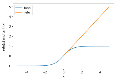
【结果分析】
- tanh函数把特征x的值压缩进-1到1的区间,-1代表x中较小的值,1代表较大的值
- relu函数把小于0的x值全部去掉,用0代替
这两种非线性处理方式,都是为了将样本特征简化,从而使神经网络可以对复杂的非线性数据集进行学习
神经网络的参数设置
在酒的数据集上使用MLP算法中的MLP分类器:
#导入MLP神经网络
from sklearn.neural_network import MLPClassifier
from sklearn.datasets import load_wine
from sklearn.model_selection import train_test_split
wine = load_wine()
X = wine.data[:,:2]
y = wine.target
#拆分数据集
X_train,X_test,y_train,y_test = train_test_split(X,y,random_state=0)
#定义分类器
mlp = MLPClassifier(solver='lbfgs') # l 是 L的小写
mlp.fit(X_train,y_train)
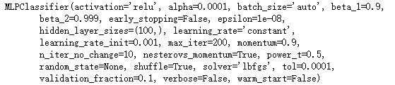
各个参数的含义:
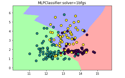
用图像展示下MLP分类的情况:
#导入画图工具
import matplotlib.pyplot as plt
from matplotlib.colors import ListedColormap
#使用不同色块表示不同分类
cmap_light = ListedColormap(['#FFAAAA','#AAFFAA','#AAAAFF'])
cmap_bold = ListedColormap(['#FF0000','#00FF00','#0000FF'])
#用样本的两个特征值创建图像和横轴和纵轴
x_min,x_max = X[:,0].min() -1,X[:,0].max() +1
y_min,y_max = X[:,1].min() -1,X[:,1].max() +1
xx,yy = np.meshgrid(np.arange(x_min,x_max,.02),np.arange(y_min,y_max,.02))
Z = mlp.predict(np.c_[(xx.ravel(),yy.ravel())])
#将每个分类中的样本分配不同的颜色
Z = Z.reshape(xx.shape)
plt.figure()
plt.pcolormesh(xx,yy,Z,cmap=cmap_light)
#将数据特征用散点图表示出来
plt.scatter(X[:,0],X[:,1],c=y,edgecolor='k',s=60)
plt.xlim(xx.min(),xx.max())
plt.ylim(yy.min(),yy.max())
plt.title('MLPClassifier:solver=1bfgs')
plt.show()
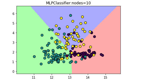
试试把隐藏层的节点变少:
#设计隐藏层中的结点数为10
mlp_20 = MLPClassifier(solver='lbfgs',hidden_layer_sizes=[10])
mlp_20.fit(X_train,y_train)
Z1 = mlp_20.predict(np.c_[xx.ravel(),yy.ravel()])
Z1 = Z1.reshape(xx.shape)
plt.figure()
plt.pcolormesh(xx,yy,Z1,cmap=cmap_light)
#用散点图画出X
plt.scatter(X[:,0],X[:,1],c=y,edgecolor='k',s=60)
plt.xlim(xx.min(),xx.max())
plt.ylim(yy.min(),yy.max())
plt.title('MLPClassifier:nodes=10')
plt.show()

给MLP分类器增加隐藏层数量:
#设计神经网络有两个节点数为10的隐藏层
mlp_2L = MLPClassifier(solver='lbfgs',hidden_layer_sizes=[10,10])
mlp_2L.fit(X_train,y_train)
Z0 = mlp_2L.predict(np.c_[xx.ravel(),yy.ravel()])
Z0 = Z0.reshape(xx.shape)
plt.figure()
plt.pcolormesh(xx,yy,Z0,cmap=cmap_light)
#用散点图画出X
plt.scatter(X[:,0],X[:,1],c=y,edgecolor='k',s=60)
plt.xlim(xx.min(),xx.max())
plt.ylim(yy.min(),yy.max())
plt.title('MLPClassifier:2Layers')
plt.show()
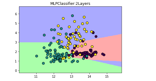
【结果分析】
隐藏层的增加的结果就是决定边界看起来更细腻
使用activation='tanh'实验:
#设计激活函数为tanh
mlp_tanh = MLPClassifier(solver='lbfgs',hidden_layer_sizes=[10,10],activation='tanh')
mlp_tanh.fit(X_train,y_train)
Z2 = mlp_tanh.predict(np.c_[xx.ravel(),yy.ravel()])
Z2 = Z2.reshape(xx.shape)
plt.figure()
plt.pcolormesh(xx,yy,Z2,cmap=cmap_light)
#用散点图画出X
plt.scatter(X[:,0],X[:,1],c=y,edgecolor='k',s=60)
plt.xlim(xx.min(),xx.max())
plt.ylim(yy.min(),yy.max())
plt.title('MLPClassifier:2Layers with tanh')
plt.show()


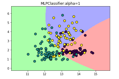
#修改模型的alpha参数
mlp_alpha = MLPClassifier(solver='lbfgs',hidden_layer_sizes=[10,10],activation='tanh',alpha=1)
mlp_alpha.fit(X_train,y_train)
Z3 = mlp_alpha.predict(np.c_[xx.ravel(),yy.ravel()])
Z3 = Z3.reshape(xx.shape)
plt.figure()
plt.pcolormesh(xx,yy,Z3,cmap=cmap_light)
#用散点图画出X
plt.scatter(X[:,0],X[:,1],c=y,edgecolor='k',s=60)
plt.xlim(xx.min(),xx.max())
plt.ylim(yy.min(),yy.max())
plt.title('MLPClassifier:alpha=1')
plt.show()

实战——手写识别
使用现成的数据集 MNIST 训练图像识别
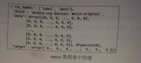
1.使用MNIST
#导入数据集获取工具
from sklearn.datasets import fetch_mldata
#加载MNIST手写数字数据集
mnist = fetch_mldata('MNIST original')
mnist

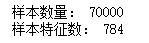
print('样本数量:',mnist.data.shape[0])
print('样本特征数:',mnist.data.shape[1])
为了控制神经网络的时长,只选5000个样本作为训练集,1000作为测试集【为了每次选取的数据保持一致,指定random_state=62】:
#建立训练集和测试集
X = mnist.data / 255
y = mnist.target
X_train,X_test,y_train,y_test = train_test_split(X,y,train_size = 5000,test_size = 1000,random_state=62)
2.训练MLP神经网络
#设置神经网络有两个100个结点的隐藏层
mlp_hw = MLPClassifier(solver='lbfgs',hidden_layer_sizes=[100,100],activation='relu',alpha=1e-5,random_state=62)
#训练神经网络模型
mlp_hw.fit(X_train,y_train)
print('测试集得分:',mlp_hw.score(X_test,y_test)*100)
测试集得分: 93.60000000000001
3.识别
#导入数据处理工具
from PIL import Image
#打开图像
image = Image.open('4.jpg').convert('F')
#调整图像大小
image = image.resize((28,28))
arr=[]
#将图像中的像素作为预测数据点的特征
for i in range(28):
for j in range(28):
pixel = 1.0-float(image.getpixel((j,i)))/255
arr.append(pixel)
#但由于只有一个样本,所以需要进行reshape操作
arr1 = np.array(arr).reshape(1,-1)
#进行图像识别
print(mlp_hw.predict(arr1)[0])

2.0
使用的图形是28*28像素:

MLP仅限于处理小数据集,对于更大或更复杂的数据集,可以进军深度学习
神经网络优点
- 计算能力充足且参数设置合适情况下,神经网络表现特优异
- 对于特征类型单一的数据,变现不错
神经网络缺点
- 训练时间长、对数据预处理要求高
- 数据特征类型差异较大,随机森林或梯度上升随机决策树算法更好


 浙公网安备 33010602011771号