机器学习项目-中文手写数字识别
最后结果展示
一、首先统计数据
%% 对读入的数据进行处理
filename = 'G:\data2\chinese_mnist.csv';
[m,raw_y] = DataOperate(filename);
1.1DataOperate函数
function [m,raw_y] = DataOperate(path)
    % 5 为变量数目
    opts = delimitedTextImportOptions("NumVariables",5);
    opts.DataLines = [2,inf]; % 数据位置DataLines 属性设置为值 [2 inf]。读取从第 5 行开始到文件末尾之间的所有数据行。
    opts.VariableNames = ["suite_id", "sample_id", "code", "value", "Var5"];
    opts.VariableTypes = ["double","double","double","double","string"];
    opts.SelectedVariableNames = ["suite_id", "sample_id", "code", "value"];

    chineseminist = table2array(readtable(path,opts)); % 将表转换为同构数组

    m = size(chineseminist,1);
    raw_y = chineseminist(randperm(m),:); % 生成一个从1到m的整数的随机排列

end
%% 定义隐层与相关数据
train_size = floor(15000 * 0.7);
width = 20;
input_layer_size  = width*width;
hidden_layer_size = 150;

num_labels = 15;
maxit = 600;
lambda = 0.03;
二、对得到的图像进行处理
%% 图像处理 读入图像并且进行裁剪
X = zeros(m,input_layer_size);

for i= 1:m
    suite_id = raw_y(i,1);
    sample_id = raw_y(i,2);
    code = raw_y(i,3);
    path = ['G:\data2\handwritingPictures\input_',mat2str(suite_id),'_',mat2str(sample_id),'_',mat2str(code),'.jpg'];
    finalimg = OperateTheImg(path,width);
    X(i,:) = reshape(finalimg,1,width*width);
end
%% 训练集 测试集划分
trainX = X(1:train_size,:);
trainY = raw_y(1:train_size,3);

testX = X(train_size+1:m,:);
testY = raw_y(train_size+1:m,3);
三、带入优化器求得超参数
%% 带入优化器求超参数
initial_Theta1 = randInitializeWeights(input_layer_size, hidden_layer_size);
initial_Theta2 = randInitializeWeights(hidden_layer_size, num_labels);

initial_nn_params = [initial_Theta1(:) ; initial_Theta2(:)];

options = optimset('MaxIter',maxit); % 将图像裁剪为20x20 输入层400 隐层150 lambda 0.03 迭代600次

costFunction = @(p) CostFunction(p,input_layer_size,hidden_layer_size,num_labels, trainX, trainY, lambda);

[nn_params, cost] = fmincg(costFunction, initial_nn_params, options);
3.1CostFunction代价函数
function [J, grad] = CostFunction(nn_params,input_layer_size,hidden_layer_size,num_labels,X, y, lambda)
    Theta1 = reshape(nn_params(1:hidden_layer_size * (input_layer_size + 1)), ...
                 hidden_layer_size, (input_layer_size + 1));

    Theta2 = reshape(nn_params((1 + (hidden_layer_size * (input_layer_size + 1))):end), ...
                 num_labels, (hidden_layer_size + 1));
	% 正向传播
    m = size(X, 1);
    X = [ones(m,1),X];
    a1 = X;
    z2 = a1*Theta1';
    a2 = sigmoid(z2);
    a2 = [ones(m,1),a2];
    z3 = a2*Theta2';
    a3 = sigmoid(z3);
    h = a3;
    % 独热编码(分类器)
    yk = zeros(m,num_labels);
    for i = 1:m
        yk(i,y(i)) = 1;
    end
	% 代价函数及正则化
    J = 1/m * sum(sum((-yk .* log(h) - (1-yk) .* log(1-h))));
    r = lambda/(2*m) * (sum(sum(Theta1(:,2:end) .^2)) + sum(sum(Theta2(:,2:end) .^ 2)) );
    J = J + r;


    % 反向传播与求梯度进行优化 不需再循环处理 按照矩阵方式进行处理
    Theta2_grad = (h - yk)' * a2 ./m + lambda/m .* Theta2;
    Theta1_grad = Theta2(:,2:end)' * (h - yk)' .* sigmoidGradient(z2') * a1 ./m + lambda /m * Theta1;
    grad = [Theta1_grad(:) ; Theta2_grad(:)];

    % 以下是通过循环方法进行反向传播 训练时间太长 训练集10500张图片 训练一次需要10500次循环共迭代600次
    % 利用反向传播法求取偏导数值,实际上这个循环可以和计算J值得循环合为一个,为了代码清晰,所以分开写了
    delta3 = zeros(num_labels,1);           %反向传播,输出层的误差
    delta2  = zeros(size(Theta1));          %反向传播,隐藏层的误差;输入层不计算误差
    for i = 1:m,                            %m为训练样本数,利用for遍历
        a1 = X(i,:)';
        z2 = Theta1 * a1;                   %对第i个训练样本正向传播得到输出h(x),即为a3
        a2 = sigmoid(z2);
        a2 = [1; a2];
        z3 = Theta2 * a2;
        a3 = sigmoid(z3);
        delta3 = a3;                        %反向传播,计算得偏导数
        delta3(y(i,:)) = delta3(y(i,:)) - 1;
        delta2 = Theta2' * delta3 .*[1;sigmoidGradient(z2)];
        delta2 = delta2(2:end);
        Theta2_grad = Theta2_grad + delta3 * a2';
        Theta1_grad = Theta1_grad + delta2 * a1';
    end
    Theta2_grad = 1/m * Theta2_grad + lambda/m * Theta2;                %正则化,修正梯度值
    Theta2_grad(:,1) = Theta2_grad(:,1) - lambda/m * Theta2(:,1);       %由于不惩罚偏执单元对应的列,所以把他减掉
    Theta1_grad = 1/m * Theta1_grad + lambda/m * Theta1;                %同理修改Theta1_grad
    Theta1_grad(:,1) = Theta1_grad(:,1) - lambda/m * Theta1(:,1);

end
3.2sigmoid函数
function g = sigmoid(z)
    g = 1.0 ./ (1.0 + exp(-z));
end
3.3sigmoidGradient 求导
function g = sigmoidGradient(z)
    g = sigmoid(z) .* (1-sigmoid(z));
end
3.4随机初始化theta
function W = randInitializeWeights(L_in, L_out)
    % theta随机初始化
    W = zeros(L_out, 1 + L_in);
    epsilon_init = 0.12;
    W = rand(L_out, 1 + L_in) * 2 * epsilon_init - epsilon_init;
end
四、预测结果
%% 重新将theta从params中取出
Theta1 = reshape(nn_params(1:hidden_layer_size * (input_layer_size + 1)), ...
hidden_layer_size, (input_layer_size + 1));
Theta2 = reshape(nn_params((1 + (hidden_layer_size * (input_layer_size + 1))):end), ...
num_labels, (hidden_layer_size + 1));
%% 对预测值进行输出(训练集/测试集)
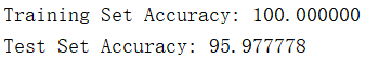
pred = predict(Theta1, Theta2, trainX);
fprintf('Training Set Accuracy: %f%\n', mean(double(pred == trainY)) * 100);
pred = predict(Theta1,Theta2,testX);
fprintf('\nTest Set Accuracy: %f%\n', mean(double(pred == testY)) * 100);
fprintf('\n');
五、对于优化器
fmincg函数
function [X, fX, i] = fmincg(f, X, options, P1, P2, P3, P4, P5)
% Minimize a continuous differentialble multivariate function. Starting point
% is given by "X" (D by 1), and the function named in the string "f", must
% return a function value and a vector of partial derivatives. The Polack-
% Ribiere flavour of conjugate gradients is used to compute search directions,
% and a line search using quadratic and cubic polynomial approximations and the
% Wolfe-Powell stopping criteria is used together with the slope ratio method
% for guessing initial step sizes. Additionally a bunch of checks are made to
% make sure that exploration is taking place and that extrapolation will not
% be unboundedly large. The "length" gives the length of the run: if it is
% positive, it gives the maximum number of line searches, if negative its
% absolute gives the maximum allowed number of function evaluations. You can
% (optionally) give "length" a second component, which will indicate the
% reduction in function value to be expected in the first line-search (defaults
% to 1.0). The function returns when either its length is up, or if no further
% progress can be made (ie, we are at a minimum, or so close that due to
% numerical problems, we cannot get any closer). If the function terminates
% within a few iterations, it could be an indication that the function value
% and derivatives are not consistent (ie, there may be a bug in the
% implementation of your "f" function). The function returns the found
% solution "X", a vector of function values "fX" indicating the progress made
% and "i" the number of iterations (line searches or function evaluations,
% depending on the sign of "length") used.
%
% Usage: [X, fX, i] = fmincg(f, X, options, P1, P2, P3, P4, P5)
%
% See also: checkgrad
%
% Copyright (C) 2001 and 2002 by Carl Edward Rasmussen. Date 2002-02-13
%
%
% (C) Copyright 1999, 2000 & 2001, Carl Edward Rasmussen
%
% Permission is granted for anyone to copy, use, or modify these
% programs and accompanying documents for purposes of research or
% education, provided this copyright notice is retained, and note is
% made of any changes that have been made.
%
% These programs and documents are distributed without any warranty,
% express or implied.  As the programs were written for research
% purposes only, they have not been tested to the degree that would be
% advisable in any important application.  All use of these programs is
% entirely at the user's own risk.
%
% [ml-class] Changes Made:
% 1) Function name and argument specifications
% 2) Output display
%

% Read options
if exist('options', 'var') && ~isempty(options) && isfield(options, 'MaxIter')
    length = options.MaxIter;
else
    length = 100;
end


RHO = 0.01;                            % a bunch of constants for line searches
SIG = 0.5;       % RHO and SIG are the constants in the Wolfe-Powell conditions
INT = 0.1;    % don't reevaluate within 0.1 of the limit of the current bracket
EXT = 3.0;                    % extrapolate maximum 3 times the current bracket
MAX = 20;                         % max 20 function evaluations per line search
RATIO = 100;                                      % maximum allowed slope ratio

argstr = ['feval(f, X'];                      % compose string used to call function
for i = 1:(nargin - 3)
  argstr = [argstr, ',P', int2str(i)];
end
argstr = [argstr, ')'];

if max(size(length)) == 2, red=length(2); length=length(1); else red=1; end
S=['Iteration '];

i = 0;                                            % zero the run length counter
ls_failed = 0;                             % no previous line search has failed
fX = [];
[f1 df1] = eval(argstr);                      % get function value and gradient
i = i + (length<0);                                            % count epochs?!
s = -df1;                                        % search direction is steepest
d1 = -s'*s;                                                 % this is the slope
z1 = red/(1-d1);                                  % initial step is red/(|s|+1)

while i < abs(length)                                      % while not finished
  i = i + (length>0);                                      % count iterations?!

  X0 = X; f0 = f1; df0 = df1;                   % make a copy of current values
  X = X + z1*s;                                             % begin line search
  [f2 df2] = eval(argstr);
  i = i + (length<0);                                          % count epochs?!
  d2 = df2'*s;
  f3 = f1; d3 = d1; z3 = -z1;             % initialize point 3 equal to point 1
  if length>0, M = MAX; else M = min(MAX, -length-i); end
  success = 0; limit = -1;                     % initialize quanteties
  while 1
    while ((f2 > f1+z1*RHO*d1) || (d2 > -SIG*d1)) && (M > 0)
      limit = z1;                                         % tighten the bracket
      if f2 > f1
        z2 = z3 - (0.5*d3*z3*z3)/(d3*z3+f2-f3);                 % quadratic fit
      else
        A = 6*(f2-f3)/z3+3*(d2+d3);                                 % cubic fit
        B = 3*(f3-f2)-z3*(d3+2*d2);
        z2 = (sqrt(B*B-A*d2*z3*z3)-B)/A;       % numerical error possible - ok!
      end
      if isnan(z2) || isinf(z2)
        z2 = z3/2;                  % if we had a numerical problem then bisect
      end
      z2 = max(min(z2, INT*z3),(1-INT)*z3);  % don't accept too close to limits
      z1 = z1 + z2;                                           % update the step
      X = X + z2*s;
      [f2 df2] = eval(argstr);
      M = M - 1; i = i + (length<0);                           % count epochs?!
      d2 = df2'*s;
      z3 = z3-z2;                    % z3 is now relative to the location of z2
    end
    if f2 > f1+z1*RHO*d1 || d2 > -SIG*d1
      break;                                                % this is a failure
    elseif d2 > SIG*d1
      success = 1; break;                                             % success
    elseif M == 0
      break;                                                          % failure
    end
    A = 6*(f2-f3)/z3+3*(d2+d3);                      % make cubic extrapolation
    B = 3*(f3-f2)-z3*(d3+2*d2);
    z2 = -d2*z3*z3/(B+sqrt(B*B-A*d2*z3*z3));        % num. error possible - ok!
    if ~isreal(z2) || isnan(z2) || isinf(z2) || z2 < 0 % num prob or wrong sign?
      if limit < -0.5                               % if we have no upper limit
        z2 = z1 * (EXT-1);                 % the extrapolate the maximum amount
      else
        z2 = (limit-z1)/2;                                   % otherwise bisect
      end
    elseif (limit > -0.5) && (z2+z1 > limit)         % extraplation beyond max?
      z2 = (limit-z1)/2;                                               % bisect
    elseif (limit < -0.5) && (z2+z1 > z1*EXT)       % extrapolation beyond limit
      z2 = z1*(EXT-1.0);                           % set to extrapolation limit
    elseif z2 < -z3*INT
      z2 = -z3*INT;
    elseif (limit > -0.5) && (z2 < (limit-z1)*(1.0-INT))  % too close to limit?
      z2 = (limit-z1)*(1.0-INT);
    end
    f3 = f2; d3 = d2; z3 = -z2;                  % set point 3 equal to point 2
    z1 = z1 + z2; X = X + z2*s;                      % update current estimates
    [f2 df2] = eval(argstr);
    M = M - 1; i = i + (length<0);                             % count epochs?!
    d2 = df2'*s;
  end                                                      % end of line search

  if success                                         % if line search succeeded
    f1 = f2; fX = [fX' f1]';
    fprintf('%s %4i | Cost: %4.6e\r', S, i, f1);
    s = (df2'*df2-df1'*df2)/(df1'*df1)*s - df2;      % Polack-Ribiere direction
    tmp = df1; df1 = df2; df2 = tmp;                         % swap derivatives
    d2 = df1'*s;
    if d2 > 0                                      % new slope must be negative
      s = -df1;                              % otherwise use steepest direction
      d2 = -s'*s;
    end
    z1 = z1 * min(RATIO, d1/(d2-realmin));          % slope ratio but max RATIO
    d1 = d2;
    ls_failed = 0;                              % this line search did not fail
  else
    X = X0; f1 = f0; df1 = df0;  % restore point from before failed line search
    if ls_failed || i > abs(length)          % line search failed twice in a row
      break;                             % or we ran out of time, so we give up
    end
    tmp = df1; df1 = df2; df2 = tmp;                         % swap derivatives
    s = -df1;                                                    % try steepest
    d1 = -s'*s;
    z1 = 1/(1-d1);
    ls_failed = 1;                                    % this line search failed
  end
  if exist('OCTAVE_VERSION')
    fflush(stdout);
  end
end
fprintf('\n');


 浙公网安备 33010602011771号